Saving and Posting Tables

On this page

library(sdvplotR)
library(gt)
library(dplyr)

A table built for a browser and a table built for a feed are not the same object. gt::gtsave() writes what the browser rendered, margins included, at whatever size the page happened to be. Posting wants a trimmed image, a predictable width across a set, and often a specific shape.

This article covers the export side of the package on one real table, the NFL’s most efficient passers of 2025, and one batch, a standings image for each AFC division: gt_save_crop(), gt_social_crop(), gt_save_batch(), the "social" density on every theme, and the two attribution functions, gt_watermark() and gt_social_tag(). The data is nflverse’s, read with nflreadr. These functions come from Andrew Weatherman’s gtUtils, and this article follows his saving guide.

Saving drives a headless Chrome through webshot2. Each save below is shown as code, and the picture under it is the image that code writes, made when this page was built.

The table

The ten quarterbacks with the most EPA per dropback (pass attempts plus sacks) among those with at least 300 dropbacks in the 2025 regular season, with NFL.com headshots and team logos.

qbs <- nflreadr::load_player_stats(2025, summary_level = "reg") |>
  filter(position == "QB") |>
  mutate(dropbacks = attempts + sacks_suffered, epa_db = passing_epa / dropbacks) |>
  filter(dropbacks >= 300) |>
  arrange(desc(epa_db), player_id) |>
  slice_head(n = 10) |>
  mutate(rank = row_number()) |>
  select(rank, player_id, player_display_name, recent_team, dropbacks, epa_db, passing_cpoe)

passers <- function(df) {
  gt(df) |>
    gt_sdv_headshots(player_id, league = "nfl", id_system = "gsis", height = 34) |>
    gt_sdv_logos(recent_team, league = "nfl", height = 24) |>
    fmt_number(epa_db, decimals = 2, force_sign = TRUE) |>
    fmt_number(passing_cpoe, decimals = 1, force_sign = TRUE) |>
    cols_label(
      rank = "", player_id = "", player_display_name = "Quarterback", recent_team = "",
      dropbacks = "Dropbacks", epa_db = "EPA/db", passing_cpoe = "CPOE"
    ) |>
    cols_align(columns = -player_display_name, "center") |>
    tab_header("The NFL's most efficient passers, 2025", "EPA per dropback, regular season, 300 or more dropbacks") |>
    tab_source_note("Data: nflverse player stats via nflreadr")
}

tbl <- gt_theme_sdv(passers(qbs))
tbl

	Quarterback	Dropbacks	EPA/db	CPOE
The NFL's most efficient passers, 2025
EPA per dropback, regular season, 300 or more dropbacks
1	Drake Maye	539	+0.31	+10.8
2	Matthew Stafford	620	+0.24	+1.5
3	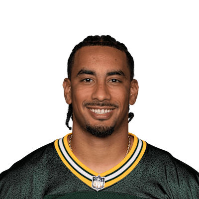Jordan Love	460	+0.24	+5.5
4	Dak Prescott	631	+0.18	+2.2
5	Jared Goff	616	+0.17	+1.8
6	Daniel Jones	406	+0.16	+2.3
7	Sam Darnold	504	+0.15	+5.2
8	Mac Jones	305	+0.15	+3.7
9	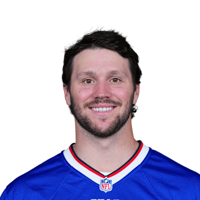Josh Allen	500	+0.14	+3.5
10	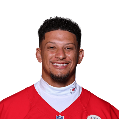Patrick Mahomes	536	+0.13	+0.3
Data: nflverse player stats via nflreadr

passers() builds the table without a theme, so each section below can dress the same rows its own way.

1. Trimming and padding

gt_save_crop() renders the table, trims the whitespace around it, then pads it back by a fixed amount so the image has an even margin on all four sides. whitespace sets that margin in pixels and bg its color, which should match the theme’s background: theme_bg records the background every theme paints.

bg <- theme_bg$bg[theme_bg$theme == "gt_theme_sdv" & theme_bg$has_style == "light"]

tbl |> gt_save_crop(file = "passers.png", bg = bg)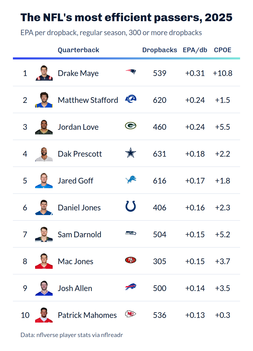

The saved image of the passers table: ten quarterbacks with headshots and team logos, trimmed and padded evenly on a white background.

zoom controls the render scale, at 2 by default, so the output is retina-sized. width is the one to know about for a series: passing it scales the finished image to an exact pixel width, holding the aspect ratio, so every image in a set lines up.

tbl |> gt_save_crop(file = "passers.png", bg = bg, width = 1080)

Leave file unset and the image is returned rather than written, which is useful when you want to keep working on it with magick.

2. Sizing type for an image

Type sized for a browser reads small once the image is scaled into a feed. Every theme in the package takes a density argument, and "social" is the setting built for this (larger body type, roomier rows, and a larger title).

qbs |>
  slice_head(n = 5) |>
  passers() |>
  gt_theme_sdv(density = "social")

	Quarterback	Dropbacks	EPA/db	CPOE
The NFL's most efficient passers, 2025
EPA per dropback, regular season, 300 or more dropbacks
1	Drake Maye	539	+0.31	+10.8
2	Matthew Stafford	620	+0.24	+1.5
3	Jordan Love	460	+0.24	+5.5
4	Dak Prescott	631	+0.18	+2.2
5	Jared Goff	616	+0.17	+1.8
Data: nflverse player stats via nflreadr

3. A fixed canvas

Some destinations want a shape rather than a size. gt_social_crop() centers the table on a canvas of a target aspect ratio. Here the top five, at social density, go on a 4:5 portrait canvas.

qbs |>
  slice_head(n = 5) |>
  passers() |>
  gt_theme_sdv(density = "social") |>
  gt_social_crop(aspect_ratio = "4:5", bg = bg, file = "passers-4x5.png")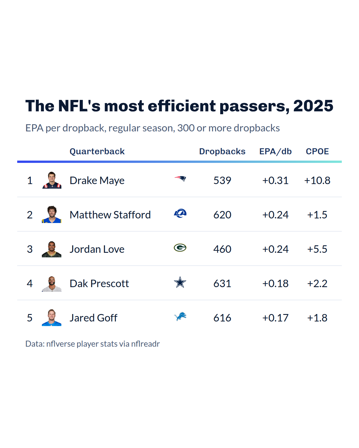

The top five passers saved as a 4:5 portrait image, the table centered on a white canvas with room above and below it.

aspect_ratio reads "1:1", "16:9", "4x5", or a bare number like 1.91. The canvas always grows to fit: it keeps the table’s size and widens or lengthens the canvas around it, so the table is never cropped to make the ratio. gravity moves the table on the canvas if you do not want it centered.

4. Attribution

gt_watermark() puts a faint wordmark behind the table body, and gt_social_tag() puts handles and icons in the source note.

qbs |>
  passers() |>
  gt_theme_broadsheet() |>
  gt_watermark(
    text = "sdvplotR", opacity = 0.06, size = "62%", angle = 20,
    font = "Helvetica"
  ) |>
  gt_social_tag(c(x = "@SportsDataverse", gh = "sportsdataverse"),
    caption = "Built with sdvplotR"
  ) |>
  gt_save_crop(file = "passers-branded.png", bg = "#FBFAF7")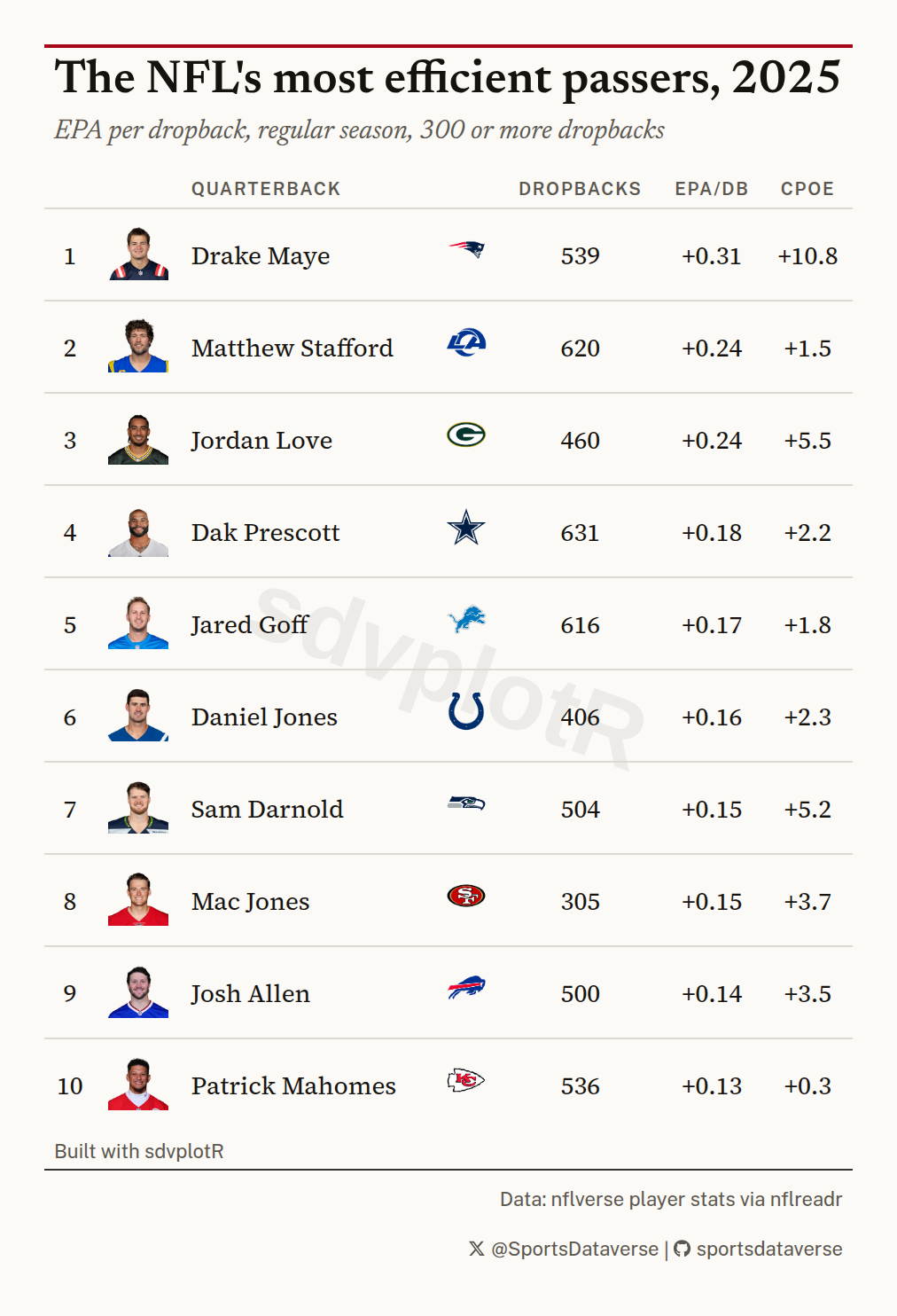

The passers table on a cream broadsheet theme with a faint sdvplotR watermark across the rows and a footer with an X handle and a GitHub name.

Two things about the watermark.

It is drawn as an SVG background image, because that is the only way to sit behind the body without taking up a row. An SVG background cannot load the page’s webfonts, so font has to name a face installed on the machine doing the rendering. "Helvetica" and "Arial" are safe. A Google font named there will silently fall back.

It also sits behind the body cells, so it disappears under any cell that has its own fill. On a striped theme, or after gt_color_ranks(), you will only see it in the gaps. Themes without fills, like gt_theme_broadsheet() or gt_theme_swiss(), show it cleanly.

gt_social_tag() takes a named vector where the names pick the icon. It knows the common aliases (x, bsky, ig, gh, yt, web, email among others) and falls back to any Font Awesome icon name. stack = TRUE puts one account per line for a narrow table.

5. One image per group

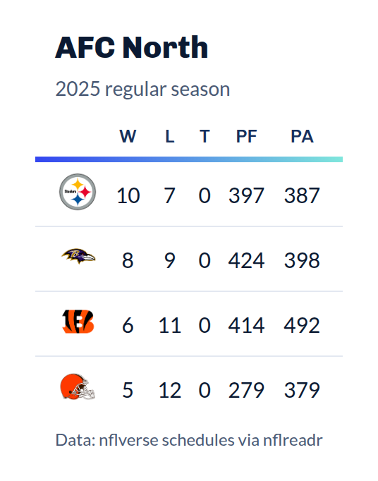
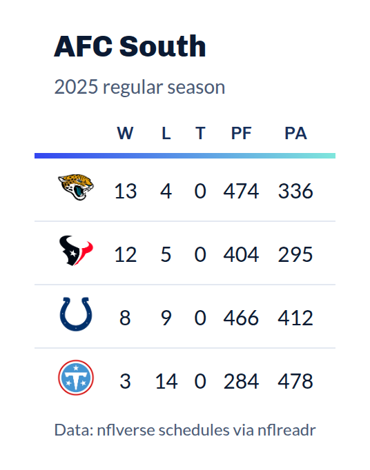
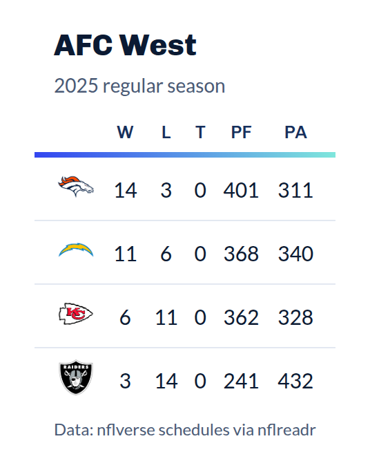
gt_save_batch() splits the data, builds a table for each group with a function you supply, and writes one image per group. The groups here are the four AFC divisions: each team’s 2025 regular-season record from the schedule, its division from nflreadr::load_teams().

nfl_teams <- nflreadr::load_teams()

records <- nflreadr::load_schedules(2025) |>
  filter(game_type == "REG", !is.na(home_score)) |>
  select(home_team, away_team, home_score, away_score) |>
  nflreadr::clean_homeaway() |>
  summarise(
    w = sum(team_score > opponent_score),
    l = sum(team_score < opponent_score),
    t = sum(team_score == opponent_score),
    pf = sum(team_score),
    pa = sum(opponent_score),
    .by = team
  ) |>
  mutate(division = nfl_teams$team_division[match(team, nfl_teams$team_abbr)]) |>
  filter(startsWith(division, "AFC")) |>
  arrange(division, desc(w + t / 2), team)

division_table <- function(df, division) {
  df |>
    select(team, w, l, t, pf, pa) |>
    gt() |>
    gt_sdv_logos(team, league = "nfl", height = 28) |>
    cols_label(team = "", w = "W", l = "L", t = "T", pf = "PF", pa = "PA") |>
    cols_align(columns = everything(), "center") |>
    tab_header(division, "2025 regular season") |>
    tab_source_note("Data: nflverse schedules via nflreadr") |>
    gt_theme_sdv()
}

division_table() receives one group’s rows and the group’s value, and returns a gt_tbl; anything else raises an error naming what came back instead. Teams are ordered by record with the abbreviation as a tiebreaker, not by the NFL’s tiebreaking rules, so the table shows no rank.

gt_save_batch(
  records,
  group = division,
  fn = division_table,
  file = "{group}.png",
  dir = "afc"
)

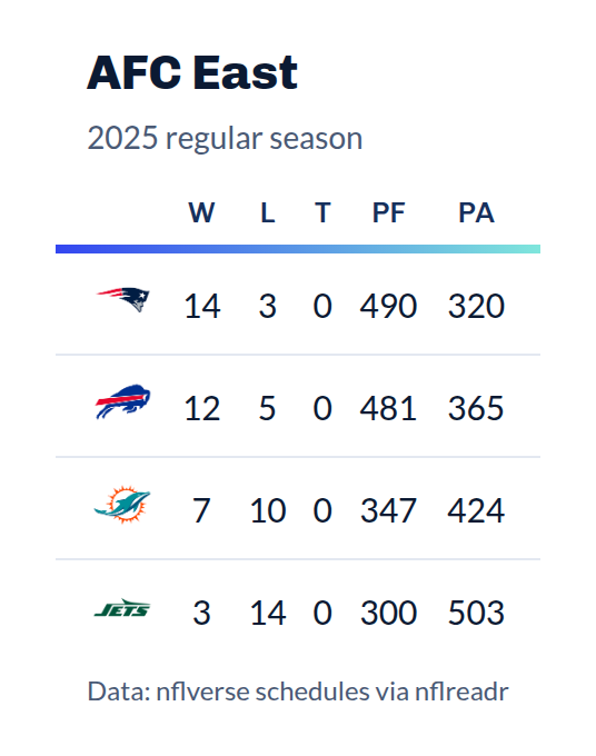
A standings image for one AFC division: four team logos with wins, losses, ties, points for and points against.

file is a pattern rather than a path. {group} is replaced by each group’s value, made safe for a file name, so this writes one image per division. The directory is created if it does not exist.

match_width is on by default and is the reason to use this over a loop: every image is padded out to the width of the widest, so a set posted side by side lines up. Set match_width = FALSE to keep each image at its natural width, and quiet = TRUE to suppress the per-group progress messages.

Our Authors

Citation

To cite the sdvplotR R package in publications, use:

BibTeX Citation

@misc{gilani_carl_lee_kay_weatherman_sdvplotR,
  author = {Gilani, Saiem and Carl, Sebastian and Lee, Jared and Kay, Camden and Weatherman, Andrew},
  title = {sdvplotR: The SportsDataverse's R Package for Multi-League Sports Plotting.},
  url = {https://sdvplotR.sportsdataverse.org},
  year = {2026}
}

sdvplot - the Python plotting package
sdvplot-js - the JavaScript / TypeScript plotting packages
cfbfastR - college football
hoopR - men’s basketball
wehoop - women’s basketball
baseballr - baseball
fastRhockey - hockey
oddsapiR - betting odds
sportyR - playing surfaces
sportsdataverse-py - the Python package
sportsdataverse-R - the R meta-package

Saiem Gilani