Team colors and themes

On this page

Ten recipes for team colors in ggplot2 and gt: a league’s palette at a glance, one color per row of your data, team fill and outline scales, colors that clash, readable text on team-colored fills, named palettes, conference colors, dark backgrounds with dark logos, and picking a table theme. The data is one season each from the NHL (fastRhockey), the NBA, the WNBA and women’s college basketball (hoopR and wehoop), MLB (baseballr) and college football (cfbfastR), all read from SportsDataverse release files except MLB’s final standings, which come from the MLB Stats API.

library(sdvplotR)
library(ggplot2)
library(dplyr, warn.conflicts = FALSE)
library(gt)

season <- 2026 # NBA, NHL and college basketball: the 2025-26 season; MLB and WNBA: 2026

1. See a league’s palette

sdv_teams() holds every team’s two colors (color_primary, color_secondary), with its conference. Laid out in rows of 8 teams, grouped by conference (two rows each), with each team’s logo above its two swatches, it is a quick check of what a chart will look like:

nhl_ref <- sdv_teams("nhl") |>
  arrange(conference, abbr) |>
  mutate(
    band = (row_number() - 1) %/% 8 + 1,
    slot = (row_number() - 1) %% 8 + 1,
    panel = paste(conference, band),
    .by = conference
  )

swatches <- bind_rows(
  transmute(nhl_ref, panel, slot, x = slot - 0.2, color = color_primary),
  transmute(nhl_ref, panel, slot, x = slot + 0.2, color = color_secondary)
)

ggplot(nhl_ref, aes(x = slot)) +
  geom_tile(aes(x = x, y = 1, fill = color), data = swatches,
    width = 0.38, height = 0.5, colour = "grey70", linewidth = 0.2
  ) +
  geom_text(aes(y = 0.58, label = paste(color_primary, color_secondary, sep = "
")), size = 2.6, lineheight = 0.95) +
  geom_sdv_logos(aes(y = 1.75, team = team_id), league = "nhl", height = 0.3) +
  scale_fill_identity() +
  facet_wrap(~panel, ncol = 1, labeller = as_labeller(function(x) ifelse(endsWith(x, " 1"), sub(" 1$", "", x), ""))) +
  scale_y_continuous(limits = c(0.3, 2.15)) +
  labs(title = "NHL team colors by conference", caption = "Colors: sdvplotR::sdv_teams()") +
  theme_void() +
  theme(strip.text = element_text(face = "bold", hjust = 0), plot.margin = margin(8, 8, 8, 8))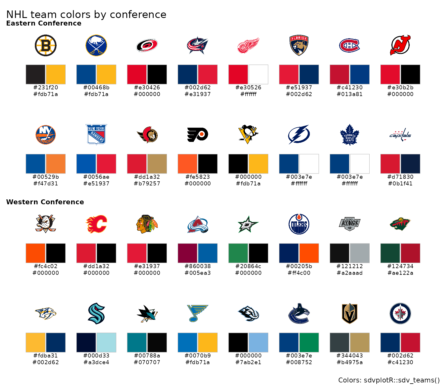

The 32 NHL teams in four rows of 8, grouped by conference: the Eastern Conference in the top two rows, the Western Conference in the bottom two. Each team's logo sits above two squares filled with its primary and secondary colors, with its two hex codes (primary above secondary) underneath.

sdv_team_colors("nhl", which = "all") returns the same pairs as "primary, secondary" strings, named by team.

2. One color per row of your data

sdv_team_colors(league, team) returns one color per value, in the order given, so it drops straight into mutate(); which = "secondary" gives the other color. Any spelling sdv_resolve() understands works, here fastRhockey’s NHL codes (LAK, TBL). With color columns in the data, the identity scales use them as they are:

nhl_games <- fastRhockey::load_nhl_team_box(season) |>
  as.data.frame() |>
  filter(substr(game_id, 5, 6) == "02") # 02 = regular season

nhl_teams <- nhl_games |>
  summarise(gf = mean(goals), ga = mean(goals_against), .by = team_abbrev) |>
  arrange(desc(gf), team_abbrev) |>
  mutate(
    primary = unname(sdv_team_colors("nhl", team_abbrev)),
    secondary = unname(sdv_team_colors("nhl", team_abbrev, which = "secondary"))
  )
head(nhl_teams, 5)
#>   team_abbrev       gf       ga primary secondary
#> 1         COL 3.682927 2.243902 #860038   #005ea3
#> 2         CAR 3.609756 2.719512 #e30426   #000000
#> 3         PIT 3.573171 2.963415 #000000   #fdb71a
#> 4         TBL 3.536585 2.609756 #003e7e   #ffffff
#> 5         BUF 3.512195 2.695122 #00468b   #fdb71a

ggplot(nhl_teams, aes(x = gf, y = ga)) +
  geom_point(aes(fill = primary, colour = secondary), shape = 21, size = 6, stroke = 1.5) +
  ggrepel::geom_text_repel(aes(label = team_abbrev), size = 2.5, point.size = 6, seed = 1) +
  scale_fill_identity() +
  scale_colour_identity() +
  scale_y_reverse() +
  labs(
    title = "NHL goals for and against per game, 2025-26",
    x = "Goals for per game", y = "Goals against per game (reversed)",
    caption = "Data: fastRhockey::load_nhl_team_box()"
  ) +
  theme_minimal()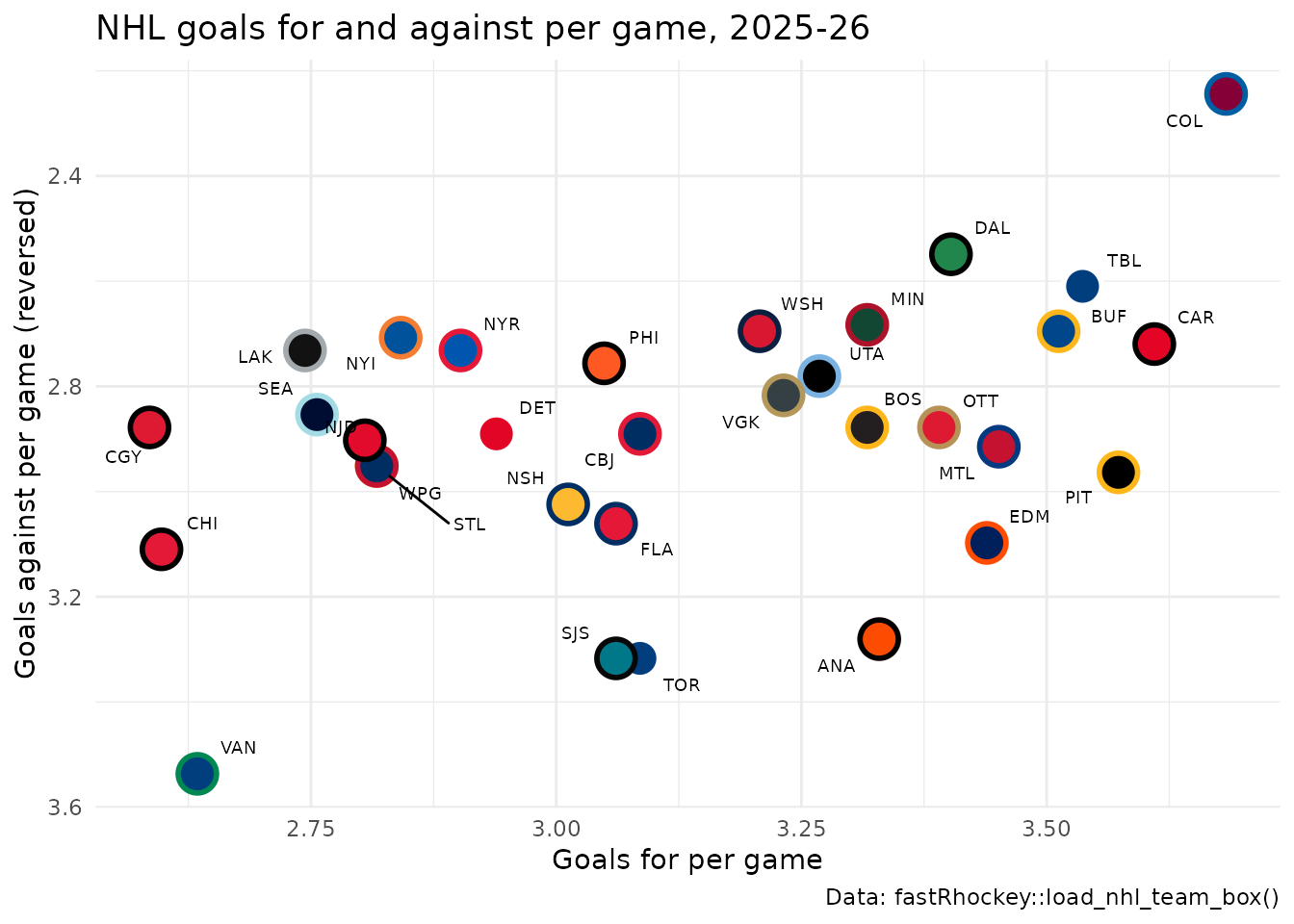

Scatter of the 32 NHL teams' goals for against goals against per game in the 2025-26 regular season. Each team is a circle filled with its primary color and outlined in its secondary color, labelled with its abbreviation.

The labels come from ggrepel, which keeps them off each other and off the points. A team that doesn’t resolve gets NA, which the identity scales draw grey; check with sdv_teams()$abbr before you publish. A white secondary, like the Lightning’s, disappears as an outline on a white chart (recipe 4).

3. Fill with the primary, outline with the secondary

scale_fill_sdv() and scale_colour_sdv() map a team column straight to colors, no join needed. Fill with the primary and outline with the secondary (which = "secondary") for the two-color look of a team’s uniform. The WNBA’s 2026 regular season by point differential. ESPN files the All-Star Game and the Commissioner’s Cup final as regular-season games too, so keep the games the schedule marks as standard (type_abbreviation == "STD"):

wnba_regular <- wehoop::load_wnba_schedule(season) |>
  as.data.frame() |>
  filter(season_type == 2, type_abbreviation == "STD") |>
  pull(game_id)
wnba <- wehoop::load_wnba_team_box(season) |>
  as.data.frame() |>
  filter(game_id %in% wnba_regular) |>
  summarise(
    games = n(),
    pf = mean(team_score),
    pa = mean(opponent_team_score),
    .by = team_abbreviation
  ) |>
  mutate(diff = pf - pa, team = team_abbreviation) |>
  arrange(desc(diff), team) |>
  mutate(team_f = factor(team, levels = team))

ggplot(wnba, aes(x = team_f, y = diff)) +
  geom_col(aes(fill = team, colour = team), width = 0.7, linewidth = 1.2) +
  geom_hline(yintercept = 0, colour = "grey30") +
  geom_sdv_logos(aes(y = diff + if_else(diff >= 0, 1.4, -1.4), team = team), league = "wnba", width = 0.05) +
  scale_fill_sdv(league = "wnba") +
  scale_colour_sdv(league = "wnba", which = "secondary") +
  labs(
    title = "WNBA point differential, 2026 regular season",
    x = NULL, y = "Average point differential per game",
    caption = "Data: wehoop::load_wnba_team_box()"
  ) +
  theme_minimal() +
  theme(axis.text.x = element_blank(), panel.grid.major.x = element_blank())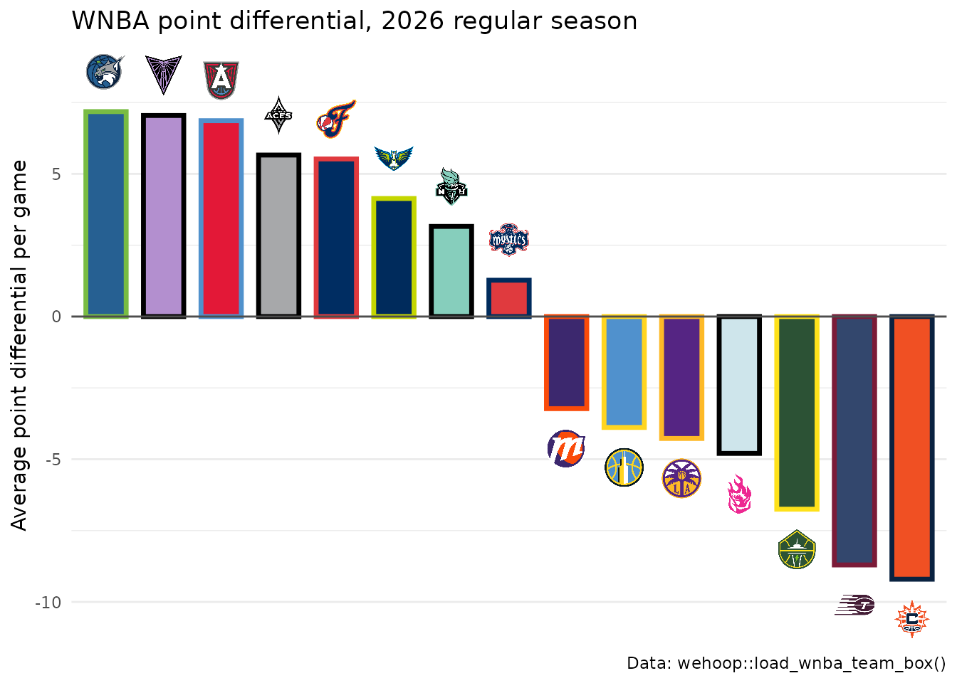

Bar chart of the 15 WNBA teams' average point differential per game in the 2026 regular season, sorted, each bar filled with the team's primary color and outlined in its secondary color, with the team's logo past the end of the bar.

alpha = on either scale fades the colors, which helps when a logo sits on the bar.

4. When two teams’ colors clash

Some rivals share a color: the Lakers’, Kings’ and Suns’ primaries are all purple, and all three play in the NBA’s Pacific Division. Measure the gap between two colors (a plain RGB distance does the job) and fall back to a team’s secondary when its primary is too close to one already used. Walk the teams best record first, so the leaders keep their primaries:

color_gap <- function(a, b) {
  m <- grDevices::col2rgb(c(a, b)) / 255
  sqrt(sum((m[, 1] - m[, 2])^2)) / sqrt(3) # 0 = same color, 1 = black vs white
}

pacific <- c("GS", "LAC", "LAL", "PHX", "SAC") # the NBA's Pacific Division
nba_regular <- hoopR::load_nba_schedule(season) |>
  as.data.frame() |>
  filter(season_type == 2, type_abbreviation == "STD") |> # no All-Star or NBA Cup final
  pull(game_id)
runs <- hoopR::load_nba_team_box(season) |>
  as.data.frame() |>
  filter(game_id %in% nba_regular, team_abbreviation %in% pacific) |>
  arrange(team_abbreviation, game_date, game_id) |>
  mutate(game_no = row_number(), wins = cumsum(team_winner), .by = team_abbreviation) |>
  rename(team = team_abbreviation)
finish <- runs |>
  slice_max(game_no, n = 1, by = team) |>
  arrange(desc(wins), team)

chosen <- character()
for (team in finish$team) {
  primary <- sdv_team_colors("nba", team)
  close <- length(chosen) > 0 && min(vapply(chosen, color_gap, numeric(1), b = primary)) < 0.15
  chosen[team] <- if (close) sdv_team_colors("nba", team, which = "secondary") else primary
}
data.frame(
  team = finish$team,
  primary = unname(sdv_team_colors("nba", finish$team)),
  used = unname(chosen[finish$team])
)
#>   team primary    used
#> 1  LAL #552583 #552583
#> 2  PHX #29127a #e56020
#> 3  LAC #12173f #12173f
#> 4   GS #fdb927 #fdb927
#> 5  SAC #5a2d81 #6a7a82

end <- max(finish$game_no)
# keep line-end logos one logo height apart (see the logos cookbook)
finish <- arrange(finish, wins, team)
finish$spot <- Reduce(function(below, y) max(y, below + 5), finish$wins, accumulate = TRUE)

ggplot(runs, aes(x = game_no, y = wins)) +
  geom_line(aes(colour = team), linewidth = 1) + # colour here only: on the logos it would tint them
  geom_segment(aes(x = game_no, xend = end + 2, y = wins, yend = spot),
    data = finish, colour = "grey60", linewidth = 0.3
  ) +
  geom_sdv_logos(aes(x = end + 5, y = spot, team = team), data = finish, league = "nba", height = 0.08) +
  scale_colour_manual(values = chosen, guide = "none") +
  scale_x_continuous(limits = c(0, end + 8)) +
  labs(
    title = "The Pacific Division's 2025-26 race",
    x = "Game", y = "Wins",
    caption = "Data: hoopR::load_nba_team_box()"
  ) +
  theme_minimal()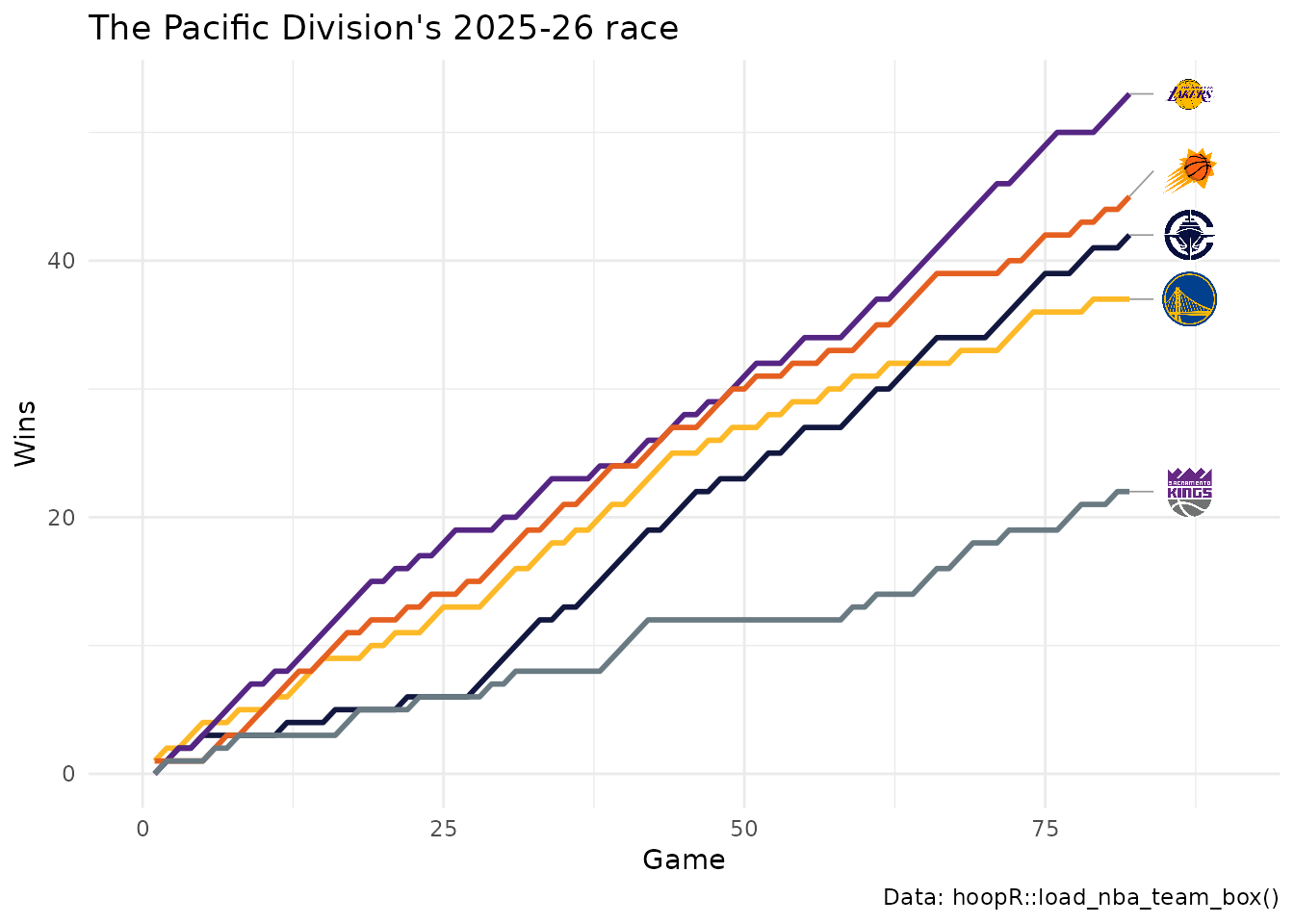

Line chart of the five NBA Pacific Division teams' cumulative wins across the 2025-26 regular season. Lines use each team's primary color, except where it was too close to a color already used, which switches to the team's secondary; each line ends in the team's logo.

A secondary is not always safe either: the Celtics’ is white, which vanishes on a white chart. Run the same check against the background.

5. Readable text on team-colored fills

Text on a team color needs the right ink: white on navy, black on gold. Pick it from the fill’s relative luminance (the WCAG formula): above 0.179, black text contrasts more than white. MLB’s 2026 regular season, wins printed inside each bar:

ink <- function(fill) {
  rgb <- grDevices::col2rgb(fill) / 255
  linear <- ifelse(rgb <= 0.04045, rgb / 12.92, ((rgb + 0.055) / 1.055)^2.4)
  luminance <- colSums(linear * c(0.2126, 0.7152, 0.0722))
  ifelse(luminance > 0.179, "black", "white")
}

mlb_ids <- baseballr::mlb_teams(season = season, sport_ids = 1) |>
  as.data.frame() |>
  select(team_records_team_id = team_id, team_abbreviation)
mlb <- baseballr::mlb_standings(season = season, league_id = "103,104") |>
  as.data.frame() |>
  inner_join(mlb_ids, by = "team_records_team_id") |>
  transmute(
    team = sdv_resolve(team_abbreviation, league = "mlb"),
    wins = team_records_wins,
    games = team_records_games_played
  ) |>
  arrange(wins, desc(team)) |>
  mutate(
    team_f = factor(team, levels = team),
    fill = unname(sdv_team_colors("mlb", team)),
    text = ink(fill)
  )
range(mlb$games)
#> [1] 161 162

ggplot(mlb, aes(x = wins, y = team_f)) +
  geom_col(aes(fill = fill), width = 0.75) +
  geom_text(aes(label = wins, colour = text), hjust = 1.3, size = 3.2, fontface = "bold") +
  scale_fill_identity() +
  scale_colour_identity() +
  scale_y_discrete(labels = NULL) +
  geom_sdv_logos(aes(x = -4, team = team), league = "mlb", height = 0.028) +
  labs(
    title = "MLB wins, 2026 regular season",
    x = "Wins", y = NULL,
    caption = "Data: baseballr::mlb_standings() (MLB Stats API)"
  ) +
  theme_minimal() +
  theme(panel.grid.major.y = element_blank())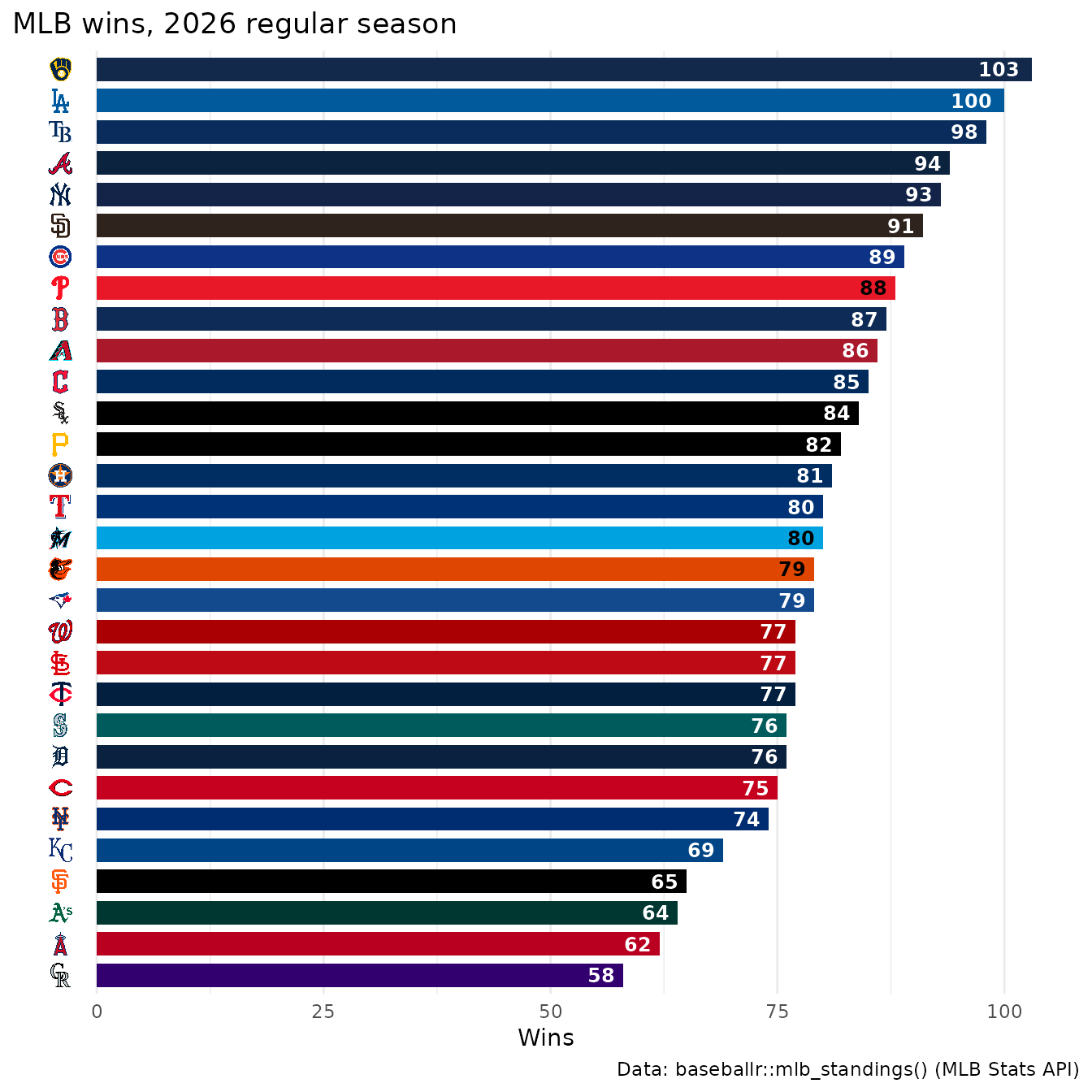

Horizontal bar chart of the 30 MLB teams' wins in the 2026 regular season, sorted, each bar filled with the team's primary color and the win total printed inside the end of the bar in black or white, whichever reads better on that color.

In a gt table, gt::data_color() picks the ink for you (autocolor_text, on by default), and gt_theme_sdv_team() does the same for its header (see recipe 10).

6. A named palette for a manual scale

sdv_color_palette(league, teams) returns a named vector of hex codes, the shape scale_colour_manual(values = ) wants. The SEC’s 2025 season, one dot per game by final margin, teams ordered by their average:

sec <- sdv_teams("cfb") |>
  filter(conference_id == "cfb:sec") |>
  pull(abbr)

cfb <- cfbfastR::load_espn_cfb_schedules(2025) |> as.data.frame()
margins <- bind_rows(
  transmute(cfb, game_id, team = home_abbreviation, margin = home_score - away_score),
  transmute(cfb, game_id, team = away_abbreviation, margin = away_score - home_score)
) |>
  filter(team %in% sec)
order <- margins |>
  summarise(avg = mean(margin), .by = team) |>
  arrange(avg, desc(team))
margins <- mutate(margins, team = factor(team, levels = order$team))

ggplot(margins, aes(x = margin, y = team, colour = team)) +
  geom_vline(xintercept = 0, colour = "grey60") +
  geom_point(size = 2.4, alpha = 0.8, position = position_jitter(width = 0, height = 0.15, seed = 1)) +
  geom_point(aes(x = avg), data = order, shape = "|", size = 6, colour = "black") +
  scale_colour_manual(values = sdv_color_palette("cfb", sec), guide = "none") +
  labs(
    title = "Every SEC game of 2025, by final margin",
    subtitle = "Black tick: each team's average margin",
    x = "Final margin (points)", y = NULL,
    caption = "Data: cfbfastR::load_espn_cfb_schedules()"
  ) +
  theme_minimal()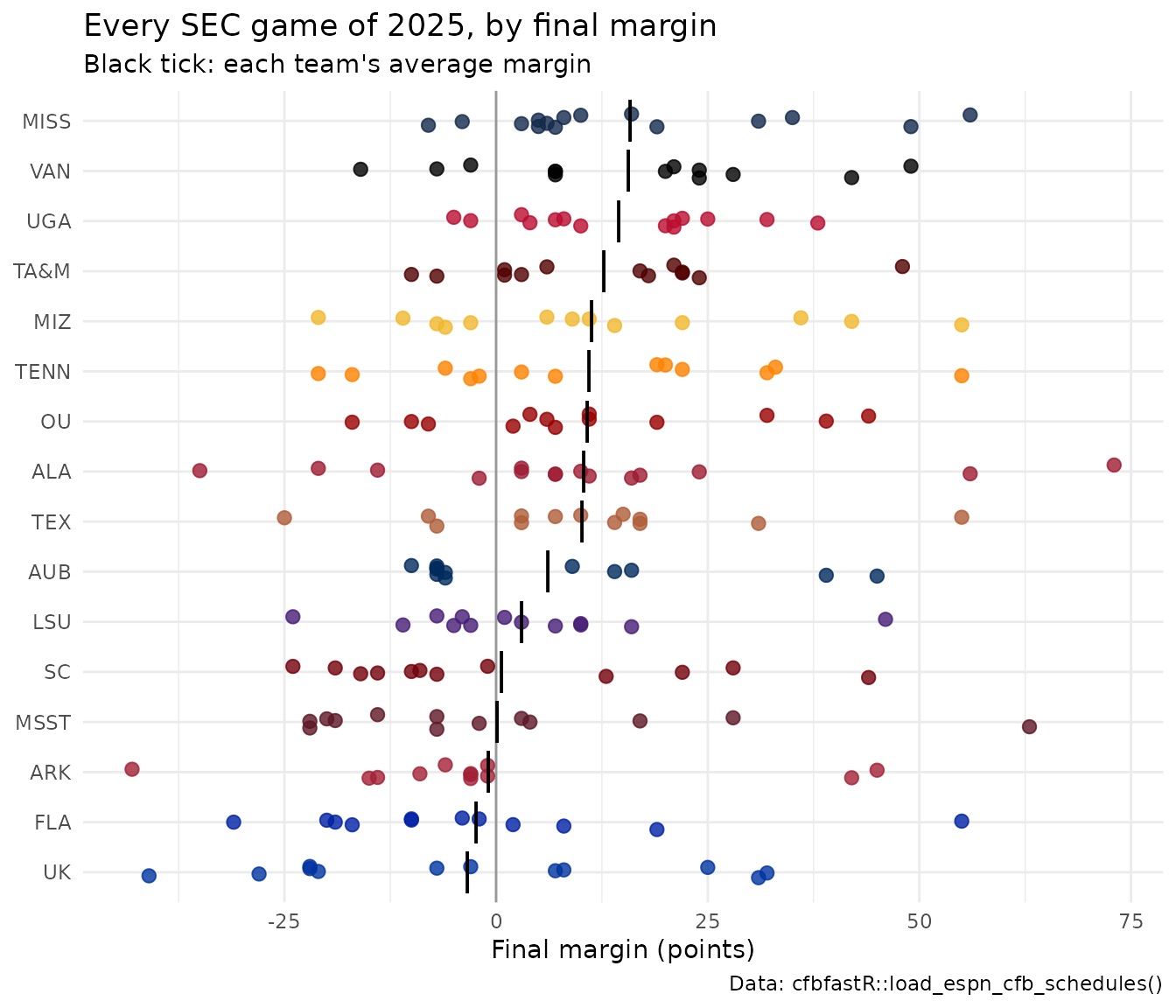

Strip plot of the 16 SEC football teams' 2025 games, one dot per game at its final scoring margin, colored in the team's primary color, with a black tick at each team's average margin. Teams are sorted by average margin, best at the top.

Several SEC primaries are near-identical crimsons and blues; across this many teams, the axis labels carry the identity and the colors only group the dots.

7. Conference colors

Conferences are rows in sdvplotR’s team index too (include_conferences = TRUE), with their colors and logos. Women’s college basketball, 2025-26: how each conference’s teams did against teams from other D-I conferences, with each season’s membership from wehoop’s standings:

wbb_conf <- wehoop::load_wbb_standings(season) |>
  as.data.frame() |>
  distinct(team_id, conference = group_name)

wbb_games <- wehoop::load_wbb_team_box(season) |>
  as.data.frame() |>
  filter(season_type == 2) |>
  inner_join(wbb_conf, by = "team_id") |>
  inner_join(rename(wbb_conf, opponent_team_id = team_id, opp_conference = conference),
    by = "opponent_team_id"
  ) |>
  filter(conference != opp_conference)

conf_rows <- sdv_teams("wbb", include_conferences = TRUE) |>
  filter(program == "conference")

nonconf <- wbb_games |>
  summarise(games = n(), win_pct = mean(team_winner), .by = conference) |>
  arrange(desc(win_pct), conference) |>
  slice_head(n = 12) |>
  mutate(
    label = sub(" Conference$", "", conference),
    label = factor(label, levels = rev(label)),
    key = conf_rows$team_id[match(conference, conf_rows$name)],
    fill = conf_rows$color_primary[match(conference, conf_rows$name)]
  )

ggplot(nonconf, aes(x = win_pct, y = label)) +
  geom_col(aes(fill = fill), width = 0.65) +
  geom_sdv_logos(aes(x = win_pct + 0.05, team = key), league = "wbb", height = 0.06) +
  scale_fill_identity() +
  scale_x_continuous(labels = scales::label_percent(), expand = expansion(mult = c(0, 0.1))) +
  labs(
    title = "Non-conference record by conference, 2025-26",
    subtitle = "Women's college basketball, regular-season games against other D-I conferences",
    x = "Win %", y = NULL,
    caption = "Data: wehoop::load_wbb_team_box(), wehoop::load_wbb_standings()"
  ) +
  theme_minimal() +
  theme(panel.grid.major.y = element_blank(), plot.title.position = "plot")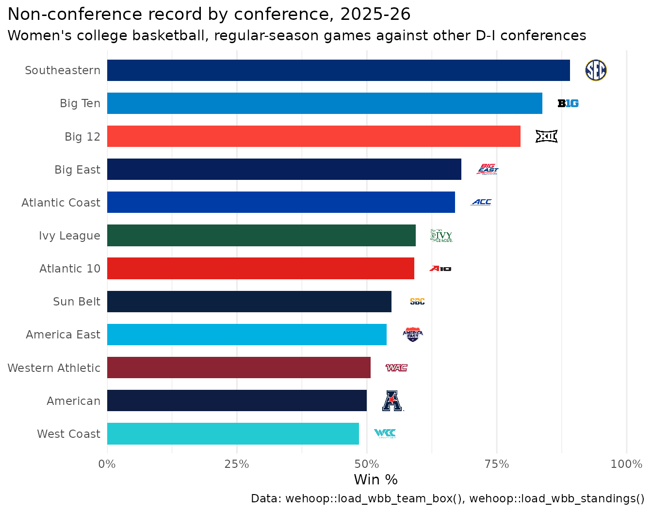

Horizontal bar chart of the twelve women's college basketball conferences with the best non-conference winning percentage in the 2025-26 regular season, each bar filled with the conference's color and ending in its logo.

sdv_teams(league, include_conferences = TRUE) lists the conference rows with their colors; sdv_logo_url() gives their logos.

8. A dark background, dark logos and a matching table

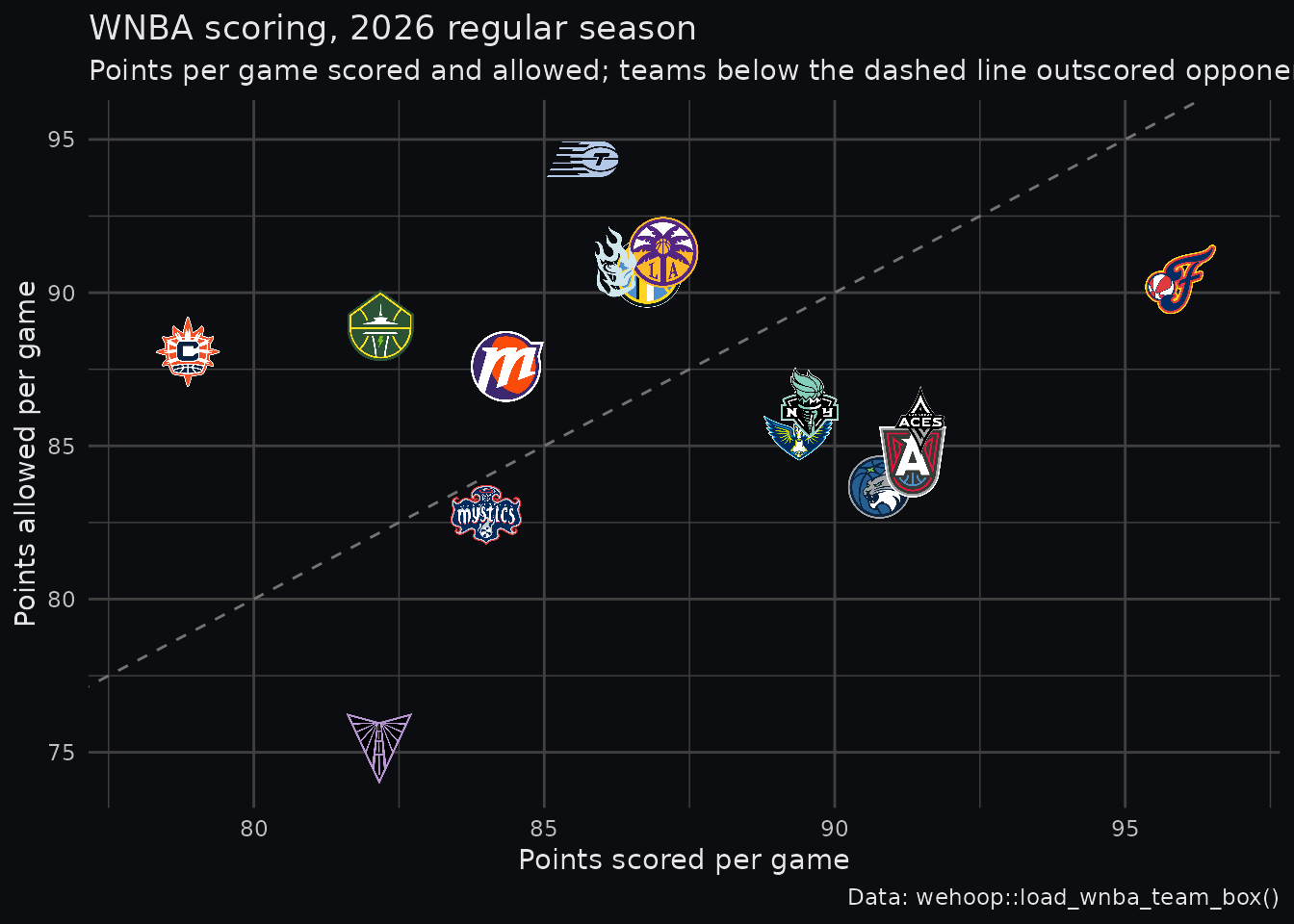
Many logos have a dark version for dark backgrounds, sdv_logo_url(variant = "dark"); draw it with geom_from_path(). theme_bg holds the background color of every gt theme, so a chart can sit on the same canvas as a table in that theme. The WNBA on gt_theme_midnight()’s background:

bg <- theme_bg$bg[theme_bg$theme == "gt_theme_midnight"]
bg
#> [1] "#0C0D10"

dark <- wnba |>
  mutate(logo_dark_url = sdv_logo_url(team, league = "wnba", variant = "dark"))

ggplot(dark, aes(x = pf, y = pa)) +
  geom_abline(slope = 1, intercept = 0, colour = "grey45", linetype = "dashed") +
  geom_from_path(aes(path = logo_dark_url), width = 0.065) +
  scale_x_continuous(expand = expansion(mult = 0.1)) +
  scale_y_continuous(expand = expansion(mult = 0.1)) +
  labs(
    title = "WNBA scoring, 2026 regular season",
    subtitle = "Points per game scored and allowed; teams below the dashed line outscored opponents",
    x = "Points scored per game", y = "Points allowed per game",
    caption = "Data: wehoop::load_wnba_team_box()"
  ) +
  theme_minimal() +
  theme(
    plot.background = element_rect(fill = bg, colour = NA),
    text = element_text(colour = "grey90"),
    axis.text = element_text(colour = "grey75"),
    panel.grid = element_line(colour = "grey25")
  )

Scatter of the 15 WNBA teams' points scored against points allowed per game in the 2026 regular season on a near-black background, each team drawn with its dark-background logo, with light grey text and grid lines.

dark |>
  arrange(desc(diff), team) |>
  head(5) |>
  select(team, pf, pa, diff) |>
  gt() |>
  gt_sdv_logos(columns = team, league = "wnba") |>
  fmt_number(columns = c(pf, pa, diff), decimals = 1) |>
  cols_label(team = "", pf = "Scored", pa = "Allowed", diff = "Margin") |>
  tab_header(title = "The WNBA's best margins, 2026") |>
  gt_theme_midnight()

	Scored	Allowed	Margin
The WNBA's best margins, 2026
	90.8	83.7	7.2
	82.2	75.1	7.0
	91.3	84.5	6.9
	91.5	85.8	5.7
	96.0	90.4	5.5

gt_sdv_logos() draws the regular logos; in a reactable table, reactable_sdv_logos(variant = "dark") picks the dark ones.

9. Choose a gt theme

gt_theme_preview() renders the same rows in several themes side by side, so you can pick one by eye before styling the full table. The NHL’s top scoring teams in six themes:

nhl_top <- nhl_teams |>
  transmute(Team = team_abbrev, `GF/G` = round(gf, 2), `GA/G` = round(ga, 2)) |>
  head(5)

gt_theme_preview(
  nhl_top,
  themes = c(
    "gt_theme_sdv", "gt_theme_athletic", "gt_theme_kenpom",
    "gt_theme_savant", "gt_theme_broadsheet", "gt_theme_midnight"
  ),
  ncol = 3
)

sdv

Team	GF/G	GA/G
COL	3.68	2.24
CAR	3.61	2.72
PIT	3.57	2.96
TBL	3.54	2.61
BUF	3.51	2.70

athletic

Team	GF/G	GA/G
COL	3.68	2.24
CAR	3.61	2.72
PIT	3.57	2.96
TBL	3.54	2.61
BUF	3.51	2.70

kenpom

toss_out_spanner_dev
Team	GF/G	GA/G
COL	3.68	2.24
CAR	3.61	2.72
PIT	3.57	2.96
TBL	3.54	2.61
BUF	3.51	2.70

savant

Team	GF/G	GA/G
COL	3.68	2.24
CAR	3.61	2.72
PIT	3.57	2.96
TBL	3.54	2.61
BUF	3.51	2.70

broadsheet

Team	GF/G	GA/G
COL	3.68	2.24
CAR	3.61	2.72
PIT	3.57	2.96
TBL	3.54	2.61
BUF	3.51	2.70

midnight

Team	GF/G	GA/G
COL	3.68	2.24
CAR	3.61	2.72
PIT	3.57	2.96
TBL	3.54	2.61
BUF	3.51	2.70

Leave themes out to see every theme in the package; file = saves the grid as one PNG (it needs a headless Chrome, through webshot2).

10. A table in a team’s colors

gt_theme_sdv_team() dresses a table in one team’s colors, with header text in whichever ink reads on them. The team with the NBA’s best point differential, and its top scorers:

players <- hoopR::load_nba_player_box(season) |>
  as.data.frame() |>
  filter(game_id %in% nba_regular, !did_not_play)

best <- players |>
  distinct(game_id, team_abbreviation, team_score, opponent_team_score) |>
  summarise(diff = mean(team_score - opponent_team_score), .by = team_abbreviation) |>
  slice_max(diff, n = 1, with_ties = FALSE) |>
  pull(team_abbreviation)

players |>
  filter(team_abbreviation == best) |>
  summarise(
    games = n(), ppg = mean(points), rpg = mean(rebounds), apg = mean(assists),
    .by = c(athlete_id, athlete_display_name)
  ) |>
  filter(games >= 20) |>
  arrange(desc(ppg), athlete_id) |>
  head(6) |>
  gt() |>
  gt_sdv_headshots(columns = athlete_id, league = "nba") |>
  fmt_number(columns = c(ppg, rpg, apg), decimals = 1) |>
  cols_label(
    athlete_id = "", athlete_display_name = "Player", games = "GP",
    ppg = "PTS", rpg = "REB", apg = "AST"
  ) |>
  tab_header(
    title = paste(sdv_teams("nba")$name[sdv_teams("nba")$abbr == best], "top scorers"),
    subtitle = "2025-26 regular season, per game, 20+ games"
  ) |>
  tab_source_note("Data: hoopR::load_nba_player_box()") |>
  gt_theme_sdv_team(team = best, league = "nba")

	Player	GP	PTS	REB	AST
Oklahoma City Thunder top scorers
2025-26 regular season, per game, 20+ games
	Shai Gilgeous-Alexander	68	31.1	4.3	6.6
	Chet Holmgren	69	17.1	8.9	1.7
	Jalen Williams	33	17.1	4.6	5.5
	Ajay Mitchell	57	13.6	3.3	3.6
	Isaiah Joe	71	11.1	2.5	1.3
	Jared McCain	31	10.1	2.0	0.9
Data: hoopR::load_nba_player_box()

gt_theme_sdv() is the house look in light or dark (style = "dark"), for tables that belong to no one team.

Our Authors

Citation

To cite the sdvplotR R package in publications, use:

BibTeX Citation

@misc{gilani_carl_lee_kay_weatherman_sdvplotR,
  author = {Gilani, Saiem and Carl, Sebastian and Lee, Jared and Kay, Camden and Weatherman, Andrew},
  title = {sdvplotR: The SportsDataverse's R Package for Multi-League Sports Plotting.},
  url = {https://sdvplotR.sportsdataverse.org},
  year = {2026}
}

sdvplot - the Python plotting package
sdvplot-js - the JavaScript / TypeScript plotting packages
cfbfastR - college football
hoopR - men’s basketball
wehoop - women’s basketball
baseballr - baseball
fastRhockey - hockey
oddsapiR - betting odds
sportyR - playing surfaces
sportsdataverse-py - the Python package
sportsdataverse-R - the R meta-package

Saiem Gilani