
CFB Conference Table
Saiem Gilani


Source: vignettes/recipe-cfb-conference-table.Rmd
recipe-cfb-conference-table.RmdOn this page
The brief: the season-review newsletter needs the final Big Ten standings as an image: 1600 px wide for the email, plus a square cut for social. Indiana went 16-0 and won the national title, so the table should make that obvious. The records are built from the CollegeFootballData.com schedule through cfbfastR, and the table is gt with sdvplotR’s logo, theme and export helpers.
library(sdvplotR)
library(gt)
library(dplyr, warn.conflicts = FALSE)

season <- 2025
conference <- "Big Ten"
out_dir <- tempfile("sdvplotR-recipe-") # where the exports go; use your own folder
dir.create(out_dir)
1. Get the data
The schedule has one row per game. Stacking the home and away sides
gives one row per team per game, which makes every record a
group_by(). The margins are kept in date order as one
comma-separated string per team, the form gt’s in-cell charts read, for
a small chart later. summarise() sees its own earlier
results, so the margins and the last game’s score are taken before
pf and pa become season averages.
schedule <- cfbfastR::load_cfb_schedules(season) |>
  filter(completed)

side <- function(me, opp) {
  transmute(
    schedule,
    start_date, season_type, conference_game, notes,
    team = .data[[paste0(me, "_team")]],
    conference = .data[[paste0(me, "_conference")]],
    opponent = .data[[paste0(opp, "_team")]],
    pf = .data[[paste0(me, "_points")]],
    pa = .data[[paste0(opp, "_points")]]
  )
}

games <- bind_rows(side("home", "away"), side("away", "home")) |>
  filter(conference == !!conference) |>
  arrange(start_date) |>
  mutate(won = pf > pa)

standings <- games |>
  group_by(team) |>
  summarise(
    margins = paste(pf - pa, collapse = ","),
    # the last game: where a bowl or the playoff shows up
    last_score = paste0(max(last(pf), last(pa)), "-", min(last(pf), last(pa))),
    last_type = last(season_type),
    last_won = last(won),
    last_opponent = last(opponent),
    last_event = last(notes),
    conf_w = sum(won & conference_game),
    conf_l = sum(!won & conference_game),
    w = sum(won),
    l = sum(!won),
    pf = mean(pf),
    pa = mean(pa)
  ) |>
  arrange(desc(conf_w), desc(w), team) # team breaks ties, so the order is the same every run
nrow(standings)
#> [1] 18
standings |>
  select(team, conf_w, conf_l, w, l, last_score, last_opponent, last_event) |>
  head(5)
#> # A tibble: 5 × 8
#>   team       conf_w conf_l     w     l last_score last_opponent last_event
#>   <chr>       <int>  <int> <int> <int> <chr>      <chr>         <chr>
#> 1 Indiana         9      0    16     0 27-21      Miami         College Footbal…
#> 2 Ohio State      9      0    12     2 24-14      Miami         College Footbal…
#> 3 Oregon          8      1    13     2 56-22      Indiana       College Footbal…
#> 4 Michigan        7      2     9     4 41-27      Texas         Cheez-It Citrus…
#> 5 USC             7      2     9     4 30-27      TCU           Valero Alamo Bo…
2. The first draft
Hand the frame to gt as it is.
gt(standings)| team | margins | last_score | last_type | last_won | last_opponent | last_event | conf_w | conf_l | w | l | pf | pa |
|---|---|---|---|---|---|---|---|---|---|---|---|---|
| Indiana | 13,47,73,53,5,10,25,50,45,3,24,53,3,35,34,6 | 27-21 | postseason | TRUE | Miami | College Football Playoff National Championship Presented by AT&T | 9 | 0 | 16 | 0 | 41.62500 | 11.687500 |
| Ohio State | 7,70,28,18,39,18,34,24,24,38,33,18,-3,-10 | 24-14 | postseason | FALSE | Miami | College Football Playoff Quarterfinal at the Goodyear Cotton Bowl Classic | 9 | 0 | 12 | 2 | 33.42857 | 9.285714 |
| Oregon | 46,66,20,34,6,-10,46,14,2,29,15,12,17,23,-34 | 56-22 | postseason | FALSE | Indiana | College Football Playoff Semifinal at the Chick-fil-A Peach Bowl | 8 | 1 | 13 | 2 | 36.93333 | 17.866667 |
| Michigan | 17,-11,60,3,14,-18,17,11,5,2,25,-18,-14 | 41-27 | postseason | FALSE | Texas | Cheez-It Citrus Bowl | 7 | 2 | 9 | 4 | 27.53846 | 20.384615 |
| USC | 60,39,16,14,-2,18,-10,4,21,5,-15,19,-3 | 30-27 | postseason | FALSE | TCU | Valero Alamo Bowl | 7 | 2 | 9 | 4 | 35.76923 | 23.000000 |
| Iowa | 27,-3,40,10,-5,37,1,38,-2,-5,3,24,7 | 34-27 | postseason | TRUE | Vanderbilt | ReliaQuest Bowl | 6 | 3 | 9 | 4 | 29.30769 | 16.076923 |
| Illinois | 49,26,38,-53,2,16,-18,-17,22,18,-17,7,2 | 30-28 | postseason | TRUE | Tennessee | Liberty Mutual Music City Bowl | 5 | 4 | 9 | 4 | 29.38462 | 23.615385 |
| Washington | 17,60,35,-18,4,19,-17,17,-3,36,34,-12,28 | 38-10 | postseason | TRUE | Boise State | Bucked Up LA Bowl | 5 | 4 | 9 | 4 | 34.07692 | 18.692308 |
| Minnesota | 13,66,-13,3,-39,7,18,-38,3,-29,-3,10,3 | 20-17 | postseason | TRUE | New Mexico | Rate Bowl | 5 | 4 | 8 | 5 | 23.00000 | 22.923077 |
| Nebraska | 3,68,52,-3,11,3,-18,7,-4,7,-27,-24,-22 | 44-22 | postseason | FALSE | Utah | SRS Distribution Las Vegas Bowl | 4 | 5 | 7 | 6 | 28.69231 | 24.615385 |
| Northwestern | -20,35,-20,3,35,1,19,-7,-21,-2,3,-7,27 | 34-7 | postseason | TRUE | Central Michigan | GameAbove Sports Bowl | 4 | 5 | 7 | 6 | 23.38462 | 19.846154 |
| Penn State | 35,34,46,-6,-5,-1,-1,-24,-3,18,27,4,12 | 22-10 | postseason | TRUE | Clemson | Bad Boy Mowers Pinstripe Bowl | 3 | 6 | 7 | 6 | 31.00000 | 20.538462 |
| UCLA | -33,-7,-25,-3,5,25,3,-50,-7,-38,-34,-19 | 29-10 | regular | FALSE | USC | NA | 3 | 6 | 3 | 9 | 18.16667 | 33.416667 |
| Rutgers | 3,28,50,-10,-3,-19,-46,3,-22,15,-33,-4 | 40-36 | regular | FALSE | Penn State | NA | 2 | 7 | 5 | 7 | 28.66667 | 31.833333 |
| Wisconsin | 17,32,-24,-17,-14,-37,-34,-14,3,-24,17,-10 | 17-7 | regular | FALSE | Minnesota | NA | 2 | 7 | 4 | 8 | 12.83333 | 21.583333 |
| Maryland | 32,11,27,17,-4,-3,-3,-45,-15,-18,-25,-10 | 38-28 | regular | FALSE | Michigan State | NA | 1 | 8 | 4 | 8 | 23.50000 | 26.500000 |
| Michigan State | 17,2,17,-14,-11,-25,-25,-11,-3,-18,-3,10 | 38-28 | regular | TRUE | Maryland | NA | 1 | 8 | 4 | 8 | 24.58333 | 29.916667 |
| Purdue | 31,17,-16,-26,-16,-7,-19,-3,-5,-24,-36,-53 | 56-3 | regular | FALSE | Indiana | NA | 0 | 9 | 2 | 10 | 18.75000 | 31.833333 |
Every number is there, and none of it is readable: margins printed as text, a dozen decimals, and column names only the analyst knows.
3. Shape it for a reader
Records read as “9-0”, not two columns. Each team’s last game becomes one short line (“W 27-21 vs Miami, CFP National Championship”), which is where the national title shows up. Columns get real labels, conference and overall records sit under spanners, and the averages get one decimal.
event <- function(x) {
  x |>
    sub(" Presented by.*", "", x = _) |>
    sub(" at the .*", "", x = _) |>
    sub("College Football Playoff", "CFP", x = _)
}

table <- standings |>
  mutate(
    conf = paste0(conf_w, "-", conf_l),
    overall = paste0(w, "-", l),
    postseason = if_else(
      last_type == "postseason",
      paste0(if_else(last_won, "W ", "L "), last_score, " vs ", last_opponent, ", ", event(last_event)),
      ""
    )
  ) |>
  select(team, conf, overall, pf, pa, margins, postseason)

draft <- gt(table) |>
  cols_hide(margins) |>
  cols_label(
    team = "Team", conf = "W-L", overall = "W-L",
    pf = "Pts/G", pa = "Opp/G", postseason = "Postseason"
  ) |>
  tab_spanner("Conference", conf) |>
  tab_spanner("Overall", c(overall, pf, pa)) |>
  fmt_number(c(pf, pa), decimals = 1) |>
  cols_align("center", c(conf, overall, pf, pa))
draft| Team |
Conference
|
Overall
|
Postseason | ||
|---|---|---|---|---|---|
| W-L | W-L | Pts/G | Opp/G | ||
| Indiana | 9-0 | 16-0 | 41.6 | 11.7 | W 27-21 vs Miami, CFP National Championship |
| Ohio State | 9-0 | 12-2 | 33.4 | 9.3 | L 24-14 vs Miami, CFP Quarterfinal |
| Oregon | 8-1 | 13-2 | 36.9 | 17.9 | L 56-22 vs Indiana, CFP Semifinal |
| Michigan | 7-2 | 9-4 | 27.5 | 20.4 | L 41-27 vs Texas, Cheez-It Citrus Bowl |
| USC | 7-2 | 9-4 | 35.8 | 23.0 | L 30-27 vs TCU, Valero Alamo Bowl |
| Iowa | 6-3 | 9-4 | 29.3 | 16.1 | W 34-27 vs Vanderbilt, ReliaQuest Bowl |
| Illinois | 5-4 | 9-4 | 29.4 | 23.6 | W 30-28 vs Tennessee, Liberty Mutual Music City Bowl |
| Washington | 5-4 | 9-4 | 34.1 | 18.7 | W 38-10 vs Boise State, Bucked Up LA Bowl |
| Minnesota | 5-4 | 8-5 | 23.0 | 22.9 | W 20-17 vs New Mexico, Rate Bowl |
| Nebraska | 4-5 | 7-6 | 28.7 | 24.6 | L 44-22 vs Utah, SRS Distribution Las Vegas Bowl |
| Northwestern | 4-5 | 7-6 | 23.4 | 19.8 | W 34-7 vs Central Michigan, GameAbove Sports Bowl |
| Penn State | 3-6 | 7-6 | 31.0 | 20.5 | W 22-10 vs Clemson, Bad Boy Mowers Pinstripe Bowl |
| UCLA | 3-6 | 3-9 | 18.2 | 33.4 | |
| Rutgers | 2-7 | 5-7 | 28.7 | 31.8 | |
| Wisconsin | 2-7 | 4-8 | 12.8 | 21.6 | |
| Maryland | 1-8 | 4-8 | 23.5 | 26.5 | |
| Michigan State | 1-8 | 4-8 | 24.6 | 29.9 | |
| Purdue | 0-9 | 2-10 | 18.8 | 31.8 | |
4. Logos and the season at a glance
gt_sdv_logos() turns the team names into logos, and
include_name = TRUE keeps the name beside each one, so the
column still reads as text. The margins string becomes a nanoplot, gt’s
in-cell bar chart: one bar per game, green for a win and red for a loss,
so a perfect season is a solid green row.
margin_bars <- nanoplot_options(
  data_bar_fill_color = "#2e8540",
  data_bar_negative_fill_color = "#c0392b",
  data_bar_stroke_color = "transparent",
  data_bar_negative_stroke_color = "transparent",
  show_data_points = FALSE,
  show_reference_line = FALSE,
  show_vertical_guides = FALSE,
  show_y_axis_guide = FALSE,
  interactive_data_values = TRUE # values on hover only, so the saved image stays clean
)

with_marks <- draft |>
  gt_sdv_logos(team, league = "cfb", height = 24, include_name = TRUE) |>
  cols_nanoplot(
    columns = margins, plot_type = "bar", autoscale = TRUE,
    new_col_name = "bars", new_col_label = "Game by game",
    after = "pa", options = margin_bars
  ) |>
  tab_spanner("Margin", bars)
with_marks| Team |
Conference
|
Overall
|
Margin
|
Postseason | ||
|---|---|---|---|---|---|---|
| W-L | W-L | Pts/G | Opp/G | Game by game | ||
 Indiana Indiana |
9-0 | 16-0 | 41.6 | 11.7 | W 27-21 vs Miami, CFP National Championship | |
 Ohio State Ohio State |
9-0 | 12-2 | 33.4 | 9.3 | L 24-14 vs Miami, CFP Quarterfinal | |
 Oregon Oregon |
8-1 | 13-2 | 36.9 | 17.9 | L 56-22 vs Indiana, CFP Semifinal | |
 Michigan Michigan |
7-2 | 9-4 | 27.5 | 20.4 | L 41-27 vs Texas, Cheez-It Citrus Bowl | |
 USC USC |
7-2 | 9-4 | 35.8 | 23.0 | L 30-27 vs TCU, Valero Alamo Bowl | |
 Iowa Iowa |
6-3 | 9-4 | 29.3 | 16.1 | W 34-27 vs Vanderbilt, ReliaQuest Bowl | |
 Illinois Illinois |
5-4 | 9-4 | 29.4 | 23.6 | W 30-28 vs Tennessee, Liberty Mutual Music City Bowl | |
 Washington Washington |
5-4 | 9-4 | 34.1 | 18.7 | W 38-10 vs Boise State, Bucked Up LA Bowl | |
 Minnesota Minnesota |
5-4 | 8-5 | 23.0 | 22.9 | W 20-17 vs New Mexico, Rate Bowl | |
 Nebraska Nebraska |
4-5 | 7-6 | 28.7 | 24.6 | L 44-22 vs Utah, SRS Distribution Las Vegas Bowl | |
 Northwestern Northwestern |
4-5 | 7-6 | 23.4 | 19.8 | W 34-7 vs Central Michigan, GameAbove Sports Bowl | |
 Penn State Penn State |
3-6 | 7-6 | 31.0 | 20.5 | W 22-10 vs Clemson, Bad Boy Mowers Pinstripe Bowl | |
 UCLA UCLA |
3-6 | 3-9 | 18.2 | 33.4 | ||
 Rutgers Rutgers |
2-7 | 5-7 | 28.7 | 31.8 | ||
 Wisconsin Wisconsin |
2-7 | 4-8 | 12.8 | 21.6 | ||
 Maryland Maryland |
1-8 | 4-8 | 23.5 | 26.5 | ||
 Michigan State Michigan State |
1-8 | 4-8 | 24.6 | 29.9 | ||
 Purdue Purdue |
0-9 | 2-10 | 18.8 | 31.8 | ||
5. Theme it and say what it means
A theme does the typography and rules in one call:
gt_theme_sdv(), the SportsDataverse house style. The title
says the news, the subtitle how to read the table, and the source note
credits the data. The champion’s row gets a soft fill in its own color
from sdv_team_colors(), and a footnote owns up to the
ordering: teams tied on conference record are listed by overall record,
which is not the conference’s tiebreaker.
champ <- standings[1, ]
stopifnot(champ$l == 0, champ$last_won, grepl("National Championship", champ$last_event))
fill <- paste0(sdv_team_colors("cfb", champ$team), "1F") # the primary color at 12% opacity

final <- with_marks |>
  tab_header(
    title = sprintf(
      "%s ran the table: %d-0 in the %s, %d-0 overall and national champion",
      champ$team, champ$conf_w, conference, champ$w
    ),
    subtitle = html(paste0(
      "Final ", season, " ", conference, " standings. Bars are each game's margin, in date order: ",
      "<span style='color:#2e8540'><b>wins</b></span> and ",
      "<span style='color:#c0392b'><b>losses</b></span>."
    ))
  ) |>
  tab_source_note("Data: CollegeFootballData.com via cfbfastR  |  Table: sdvplotR + gt") |>
  tab_footnote(
    "Teams tied on conference record are listed by overall record, then by name.",
    locations = cells_column_labels(columns = conf)
  ) |>
  tab_style(style = cell_fill(color = fill), locations = cells_body(rows = team == champ$team)) |>
  tab_style(
    style = cell_text(weight = "bold"),
    locations = cells_body(columns = team, rows = team == champ$team)
  ) |>
  gt_theme_sdv()
final| Indiana ran the table: 9-0 in the Big Ten, 16-0 overall and national champion | ||||||
| Final 2025 Big Ten standings. Bars are each game's margin, in date order: wins and losses. | ||||||
| Team |
Conference
|
Overall
|
Margin
|
Postseason | ||
|---|---|---|---|---|---|---|
| W-L1 | W-L | Pts/G | Opp/G | Game by game | ||
|
Indiana |
9-0 | 16-0 | 41.6 | 11.7 | W 27-21 vs Miami, CFP National Championship | |
|
Ohio State |
9-0 | 12-2 | 33.4 | 9.3 | L 24-14 vs Miami, CFP Quarterfinal | |
|
Oregon |
8-1 | 13-2 | 36.9 | 17.9 | L 56-22 vs Indiana, CFP Semifinal | |
|
Michigan |
7-2 | 9-4 | 27.5 | 20.4 | L 41-27 vs Texas, Cheez-It Citrus Bowl | |
|
USC |
7-2 | 9-4 | 35.8 | 23.0 | L 30-27 vs TCU, Valero Alamo Bowl | |
|
Iowa |
6-3 | 9-4 | 29.3 | 16.1 | W 34-27 vs Vanderbilt, ReliaQuest Bowl | |
|
Illinois |
5-4 | 9-4 | 29.4 | 23.6 | W 30-28 vs Tennessee, Liberty Mutual Music City Bowl | |
|
Washington |
5-4 | 9-4 | 34.1 | 18.7 | W 38-10 vs Boise State, Bucked Up LA Bowl | |
|
Minnesota |
5-4 | 8-5 | 23.0 | 22.9 | W 20-17 vs New Mexico, Rate Bowl | |
|
Nebraska |
4-5 | 7-6 | 28.7 | 24.6 | L 44-22 vs Utah, SRS Distribution Las Vegas Bowl | |
|
Northwestern |
4-5 | 7-6 | 23.4 | 19.8 | W 34-7 vs Central Michigan, GameAbove Sports Bowl | |
|
Penn State |
3-6 | 7-6 | 31.0 | 20.5 | W 22-10 vs Clemson, Bad Boy Mowers Pinstripe Bowl | |
|
UCLA |
3-6 | 3-9 | 18.2 | 33.4 | ||
|
Rutgers |
2-7 | 5-7 | 28.7 | 31.8 | ||
|
Wisconsin |
2-7 | 4-8 | 12.8 | 21.6 | ||
|
Maryland |
1-8 | 4-8 | 23.5 | 26.5 | ||
|
Michigan State |
1-8 | 4-8 | 24.6 | 29.9 | ||
|
Purdue |
0-9 | 2-10 | 18.8 | 31.8 | ||
| 1 Teams tied on conference record are listed by overall record, then by name. | ||||||
| Data: CollegeFootballData.com via cfbfastR | Table: sdvplotR + gt | ||||||
6. Export for the newsletter and for social
gt_save_crop() renders the table in headless Chrome,
trims it with an even border and, with width, scales it to
the email’s 1600 px. gt_social_crop() centers the same
table on a square canvas for Instagram, never cropping it: it pads
whichever way the table needs, side padding for a tall table and room
above and below for a wide one like this.
newsletter <- gt_save_crop(final, file.path(out_dir, "big_ten_1600.png"), width = 1600)
square <- gt_social_crop(
  final, file.path(out_dir, "big_ten_1080x1080.png"),
  aspect_ratio = "1:1", width = 1080
)
magick::image_info(magick::image_read(c(newsletter, square)))[c("width", "height")]
#> # A tibble: 2 × 2
#>   width height
#>   <int>  <int>
#> 1  1600   1456
#> 2  1080   1080
magick::image_read(newsletter)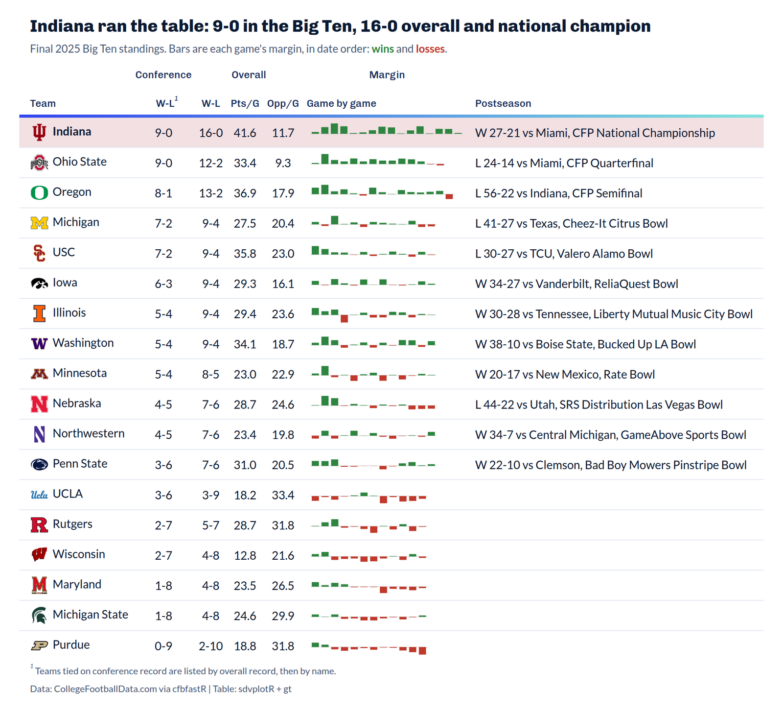
The square cut keeps the whole table and pads above and below it:
magick::image_read(square)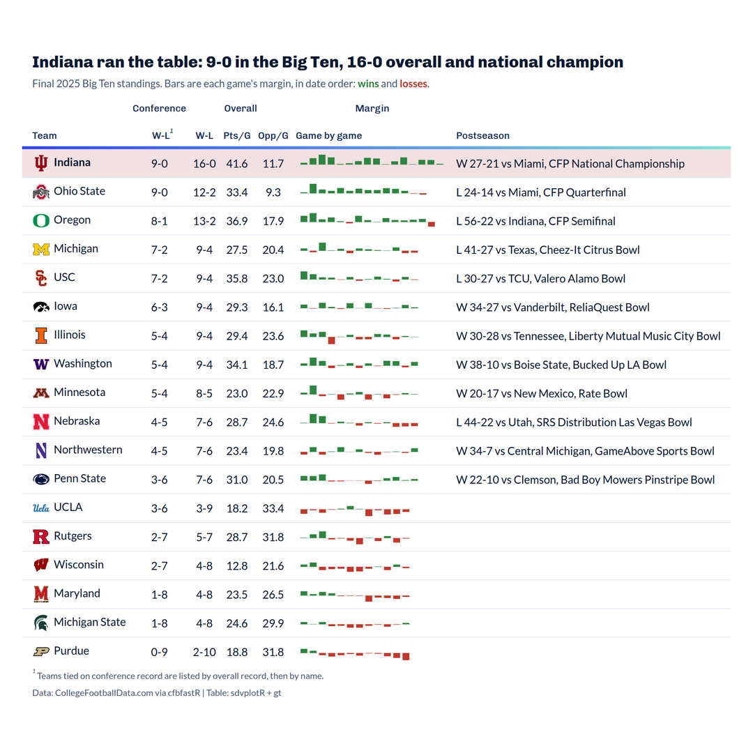






Related SportsDataverse packages
- sdvplot - the Python plotting package
- sdvplot-js - the JavaScript / TypeScript plotting packages
- cfbfastR - college football
- hoopR - men’s basketball
- wehoop - women’s basketball
- baseballr - baseball
- fastRhockey - hockey
- oddsapiR - betting odds
- sportyR - playing surfaces
- sportsdataverse-py - the Python package
- sportsdataverse-R - the R meta-package