


On this page
Every shooter has a shape: how often he shoots from each distance, and how well. This recipe draws that shape as a ribbon. The x axis is shot distance in 1 ft buckets, the ribbon’s thickness is the share of his attempts from that distance, and its fill is his field goal percentage minus the league’s from the same distance. Buckets with fewer than 10 attempts are faded, so a 3-for-4 from 31 ft does not read like a real strength.
The data
The nba_stats_metric_curves release has one file per
season and no R loader, so read it by URL with
nflreadr::load_from_url(). Its assets are named by the
season’s ending year, so 2026 is 2025-26.
url <- paste0(
  "https://github.com/sportsdataverse/sportsdataverse-data/releases/download/",
  "nba_stats_metric_curves/metric_curves_2026.rds"
)
curves <- as.data.frame(nflreadr::load_from_url(url))
stopifnot(nrow(curves) > 0)
dim(curves)
#> [1] 14881    14
count(curves, entity_type, metric)
#>   entity_type                  metric     n
#> 1      league fg_pct_by_shot_distance    37
#> 2      player fg_pct_by_shot_distance 13760
#> 3        team fg_pct_by_shot_distance  1084
Each row is one bucket of one curve: attempts,
successes and rate between x_lo
and x_hi feet, for the league, a team or a player. The
league curve is the reference:
league <- curves |>
  filter(entity_type == "league", metric == "fg_pct_by_shot_distance") |>
  select(x_lo, x_hi, league_attempts = attempts, league_rate = rate)
league
#>    x_lo x_hi league_attempts league_rate
#> 1     0    1           16067   0.7557727
#> 2     1    2           21037   0.7346580
#> 3     2    3           17128   0.6091196
#> 4     3    4           12132   0.5264590
#> 5     4    5            8569   0.4536119
#> 6     5    6            7158   0.4301481
#> 7     6    7            6276   0.4236775
#> 8     7    8            5166   0.4351529
#> 9     8    9            4874   0.4456299
#> 10    9   10            4474   0.4398748
#> 11   10   11            4391   0.4383967
#> 12   11   12            4403   0.4599137
#> 13   12   13            3971   0.4686477
#> 14   13   14            3633   0.4340765
#> 15   14   15            3058   0.4372139
#> 16   15   16            2997   0.4267601
#> 17   16   17            2630   0.4288973
#> 18   17   18            2331   0.4024024
#> 19   18   19            2010   0.4009950
#> 20   19   20            1654   0.3966143
#> 21   20   21            1276   0.3887147
#> 22   21   22             785   0.3528662
#> 23   22   23            8059   0.3762253
#> 24   23   24           14069   0.3906461
#> 25   24   25           13249   0.3742169
#> 26   25   26           26040   0.3561060
#> 27   26   27           19441   0.3476159
#> 28   27   28            9095   0.3402969
#> 29   28   29            3933   0.3325706
#> 30   29   30            1796   0.3084633
#> 31   30   31             913   0.2968237
#> 32   31   32             432   0.2916667
#> 33   32   33             211   0.2938389
#> 34   33   34             130   0.2538462
#> 35   34   35              73   0.1780822
#> 36   35   50             157   0.2738854
#> 37   50   95              14   0.5000000
The buckets are 1 ft wide out to 35 ft, then 35 to 50 and 50 to 95. Those last two are mostly end-of-quarter heaves, so the ribbon stops at 35 ft.
One shooter
Player rows carry a last name only ("Brown" names
several players), so pick the shooter by entity_id, the
stats.nba.com person id. Buckets he never shot from have no row; they
join in from the league curve as zero attempts.
shooter_id <- "1629029"
shooter <- "Luka Dončić"

mine <- curves |>
  filter(
    entity_type == "player", entity_id == shooter_id,
    metric == "fg_pct_by_shot_distance"
  )
unique(mine$entity_name)
#> [1] "Dončić"
stopifnot(nrow(mine) > 0, !anyDuplicated(mine$x_lo))

ribbon <- league |>
  filter(x_hi <= 35) |>
  left_join(select(mine, x_lo, attempts, rate), by = "x_lo") |>
  mutate(
    attempts = coalesce(attempts, 0L),
    share = attempts / sum(attempts),
    league_share = league_attempts / sum(league_attempts),
    diff = rate - league_rate,
    sample = if_else(attempts < 10, "Under 10 attempts", "10+ attempts")
  )
sum(ribbon$attempts)
#> [1] 1454
count(ribbon, sample)
#>              sample  n
#> 1      10+ attempts 30
#> 2 Under 10 attempts  5
The team colors come from the team rows, whose
entity_name is the team’s abbreviation. The file gives each
player one team_id, so a player traded mid-season still
maps to one team, but check that the lookup finds exactly one.
shooter_team <- curves |>
  filter(entity_type == "team", entity_id %in% unique(mine$team_id)) |>
  pull(entity_name) |>
  unique()
stopifnot(length(shooter_team) == 1)
shooter_team
#> [1] "LAL"
above <- sdv_team_colors("nba", shooter_team, which = "primary")
below <- sdv_team_colors("nba", shooter_team, which = "secondary")
The ribbon
Each bucket is a rectangle centred on zero, share thick.
The dashed outline is the league’s shape, for comparison. The fill runs
from the team’s secondary color (below the league) through grey to its
primary color (above the league), capped at 20 points. If a team’s
secondary color is close to grey or white, the “below” end blurs into
the midpoint: pass a darker color as below for that
team.
ggplot(ribbon) +
  geom_rect(
    aes(
      xmin = x_lo, xmax = x_hi, ymin = -share / 2, ymax = share / 2,
      fill = diff, alpha = sample
    )
  ) +
  geom_step(
    aes(x_lo, league_share / 2),
    linetype = "dashed", colour = "grey30"
  ) +
  geom_step(
    aes(x_lo, -league_share / 2),
    linetype = "dashed", colour = "grey30"
  ) +
  annotate(
    "text", x = 23.75, y = -max(ribbon$share) / 2, label = "3-pt arc",
    hjust = 1.1, vjust = 0, size = 3, colour = "grey30"
  ) +
  geom_vline(xintercept = 23.75, colour = "grey60", linewidth = 0.3) +
  scale_fill_gradient2(
    low = below, mid = "grey85", high = above, midpoint = 0,
    limits = c(-0.2, 0.2), oob = scales::squish, na.value = "grey95",
    labels = function(v) sprintf("%+.0f", 100 * v),
    name = "FG% vs league\n(points)"
  ) +
  scale_alpha_manual(
    values = c("10+ attempts" = 1, "Under 10 attempts" = 0.3), name = NULL
  ) +
  scale_x_continuous(breaks = seq(0, 35, 5), name = "Shot distance (ft)") +
  scale_y_continuous(
    labels = function(v) scales::percent(2 * abs(v), accuracy = 1),
    name = "Share of attempts\n(ribbon thickness)"
  ) +
  ggtitle_image(
    title_image = shooter_team,
    title = shooter,
    subtitle = "2025-26, 1 ft buckets to 35 ft, buckets under 10 attempts faded",
    image_height = 22,
    league = "nba"
  ) +
  labs(caption = "Data: sportsdataverse-data release nba_stats_metric_curves") +
  theme_minimal() +
  theme_title_image(size = 16) +
  theme(legend.position = "bottom", panel.grid.minor = element_blank())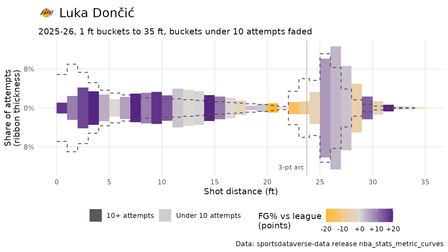






Related SportsDataverse packages
- sdvplot - the Python plotting package
- sdvplot-js - the JavaScript / TypeScript plotting packages
- cfbfastR - college football
- hoopR - men’s basketball
- wehoop - women’s basketball
- baseballr - baseball
- fastRhockey - hockey
- oddsapiR - betting odds
- sportyR - playing surfaces
- sportsdataverse-py - the Python package
- sportsdataverse-R - the R meta-package