


On this page
Updated 2026-10-12: the final 2026 regular season; the postseason is under way.
This page is rebuilt every week with the site. It builds the division standings, charts run differential with logos and lists the league leaders with their headshots, for the latest MLB season with games: the season to date from opening day to the end of September, the final regular season after that. Data: the MLB Stats API through baseballr; no key needed.
Picking the season
The season runs inside one calendar year, but before opening day the
Stats API standings for the new season come back empty, or with every
team on zero games. The helper turns both into “not published” and the
page steps back one season. Every Stats API call goes through
live(): if the API does not answer, the page shows a note
in place of each table and chart for that week instead of failing the
site build. The Stats API’s season calendar (mlb_seasons())
says whether the regular season is still being played, so the status
line can say what the numbers cover.
library(sdvplotR)
library(dplyr, warn.conflicts = FALSE)
library(ggplot2)
library(gt)

today <- Sys.Date()
current <- as.integer(format(today, "%Y")) # the season runs inside one calendar year

# A live API call, or NULL when the API does not answer: one bad week then shows
# a note in place of a table instead of failing the whole site build
live <- function(expr) tryCatch(expr, error = function(e) NULL)
unavailable <- function(what, ok) {
  if (ok) "" else sprintf("*%s were unavailable when this page was built on %s; they return next week.*", what, today)
}

# A season's standings from the MLB Stats API, or NULL before opening day: the
# API answers with no rows for a season it has no standings for, or with every
# team on zero games
standings_for <- function(season) {
  table <- live(baseballr::mlb_standings(season = season, league_id = "103,104"))
  if (NROW(table) == 0 || max(table$team_records_games_played) == 0) NULL else table
}

season <- current
raw_standings <- standings_for(season)
if (is.null(raw_standings)) {
  season <- current - 1
  raw_standings <- standings_for(season)
}
# last season always has standings, so none for either season means the API did not answer
available <- !is.null(raw_standings)
leaders_ok <- FALSE

# The Stats API's calendar for the current season: when its regular season and
# postseason end
calendar <- live(baseballr::mlb_seasons(sport_id = 1))
regular_end <- as.Date(as.character(calendar$regular_season_end_date[calendar$season_id == current]))
post_end <- as.Date(as.character(calendar$post_season_end_date[calendar$season_id == current]))
games_per_team <- if (available) round(median(raw_standings$team_records_games_played)) else NA
if (!available) {
  status <- "the MLB Stats API did not answer when this page was built, so this week's tables and chart are missing; they return next week."
  through <- ""
} else if (season < current) {
  status <- sprintf(
    "the offseason, so this is the final %d regular season; the %d season has no games yet.",
    season, current
  )
  through <- "final regular season"
} else if (length(regular_end) == 1 && today <= regular_end) {
  status <- sprintf("the %d season to date, about %d games per team.", season, games_per_team)
  through <- paste("through", games_per_team, "games")
} else if (length(post_end) == 1 && today <= post_end) {
  status <- sprintf("the final %d regular season; the postseason is under way.", season)
  through <- "final regular season"
} else {
  status <- sprintf("the offseason, so this is the final %d regular season.", season)
  through <- "final regular season"
}
The standings name each club by its nickname;
mlb_teams() adds its abbreviation, full name and division,
joined on the Stats API team id.
clubs <- live(baseballr::mlb_teams(season = season, sport_ids = 1))
available <- NROW(clubs) > 0 # mlb_teams(), like mlb_standings(), answers with no rows when the API is down
clubs <- select(clubs, team_id, abbreviation = team_abbreviation, team_name = team_full_name, division = division_name)
standings <- raw_standings |>
  transmute(
    team_id = team_records_team_id,
    rank = as.integer(team_records_division_rank),
    w = team_records_wins,
    l = team_records_losses,
    pct = as.numeric(team_records_winning_percentage),
    gb = team_records_division_games_back,
    rs = team_records_runs_scored,
    ra = team_records_runs_allowed,
    diff = team_records_run_differential,
    streak = team_records_streak_streak_code
  )
stopifnot(identical(class(standings$team_id), class(clubs$team_id)))
standings <- inner_join(standings, clubs, by = "team_id") |>
  arrange(division, rank)
nrow(standings)
#> [1] 30
1. Division standings
Six tables in one, grouped by division. gt_sdv_logos()
turns the Stats API abbreviations into logos (sdvplotR maps its
AZ and CWS to ESPN’s ARI and
CHW), and gt_color_pills() draws the run
differential on a scale centred at zero.
reach <- max(abs(standings$diff))
standings |>
  mutate(logo = abbreviation) |>
  select(division, logo, team_name, w, l, pct, gb, rs, ra, diff, streak) |>
  gt(groupname_col = "division", id = "mlb-standings") |>
  tab_header(
    title = paste("MLB standings,", season),
    subtitle = paste("By division,", through)
  ) |>
  fmt_number(pct, decimals = 3) |>
  cols_label(
    logo = "", team_name = "Team", w = "W", l = "L", pct = "Pct", gb = "GB",
    rs = "RS", ra = "RA", diff = "Diff", streak = "Streak"
  ) |>
  tab_source_note("Data: MLB Stats API via baseballr | Viz: sdvplotR") |>
  gt_color_pills(
    diff,
    palette = c("#c84630", "#f7f7f7", "#2a7ab9"), domain = c(-reach, reach),
    digits = 0, pill_height = 22
  ) |>
  gt_sdv_logos(columns = logo, league = "mlb", height = 24) |>
gt_theme_broadsheet()| MLB standings, 2026 | |||||||||
| By division, final regular season | |||||||||
| Team | W | L | Pct | GB | RS | RA | Diff | Streak | |
|---|---|---|---|---|---|---|---|---|---|
| American League Central | |||||||||
 |
Cleveland Guardians | 85 | 77 | 0.525 | - | 678 | 667 | 11 | L1 |
 |
Chicago White Sox | 84 | 78 | 0.519 | 1.0 | 776 | 720 | 56 | W1 |
 |
Minnesota Twins | 77 | 85 | 0.475 | 8.0 | 739 | 797 | -58 | W1 |
 |
Detroit Tigers | 76 | 86 | 0.469 | 9.0 | 723 | 652 | 71 | L1 |
 |
Kansas City Royals | 69 | 93 | 0.426 | 16.0 | 690 | 810 | -120 | W1 |
| American League East | |||||||||
 |
Tampa Bay Rays | 98 | 64 | 0.605 | - | 736 | 650 | 86 | L1 |
 |
New York Yankees | 93 | 68 | 0.578 | 4.5 | 739 | 601 | 138 | W1 |
 |
Boston Red Sox | 87 | 75 | 0.537 | 11.0 | 689 | 611 | 78 | L1 |
 |
Baltimore Orioles | 79 | 82 | 0.491 | 18.5 | 718 | 739 | -21 | L1 |
 |
Toronto Blue Jays | 79 | 83 | 0.488 | 19.0 | 648 | 694 | -46 | W1 |
| American League West | |||||||||
 |
Houston Astros | 81 | 81 | 0.500 | - | 734 | 766 | -32 | W2 |
 |
Texas Rangers | 80 | 82 | 0.494 | 1.0 | 673 | 719 | -46 | L1 |
 |
Seattle Mariners | 76 | 86 | 0.469 | 5.0 | 664 | 722 | -58 | W2 |
 |
Athletics | 64 | 98 | 0.395 | 17.0 | 699 | 937 | -238 | L2 |
 |
Los Angeles Angels | 62 | 100 | 0.383 | 19.0 | 655 | 752 | -97 | L2 |
| National League Central | |||||||||
 |
Milwaukee Brewers | 103 | 59 | 0.636 | - | 832 | 618 | 214 | W5 |
 |
Chicago Cubs | 89 | 73 | 0.549 | 14.0 | 850 | 703 | 147 | W1 |
 |
Pittsburgh Pirates | 82 | 80 | 0.506 | 21.0 | 767 | 739 | 28 | W1 |
 |
St. Louis Cardinals | 77 | 85 | 0.475 | 26.0 | 720 | 749 | -29 | L4 |
 |
Cincinnati Reds | 75 | 87 | 0.463 | 28.0 | 666 | 826 | -160 | L1 |
| National League East | |||||||||
 |
Atlanta Braves | 94 | 68 | 0.580 | - | 742 | 626 | 116 | L1 |
 |
Philadelphia Phillies | 88 | 74 | 0.543 | 6.0 | 713 | 698 | 15 | W1 |
 |
Miami Marlins | 80 | 82 | 0.494 | 14.0 | 715 | 712 | 3 | W1 |
 |
Washington Nationals | 77 | 85 | 0.475 | 17.0 | 821 | 815 | 6 | W1 |
 |
New York Mets | 74 | 88 | 0.457 | 20.0 | 699 | 731 | -32 | L1 |
| National League West | |||||||||
 |
Los Angeles Dodgers | 100 | 62 | 0.617 | - | 801 | 600 | 201 | W3 |
 |
San Diego Padres | 91 | 71 | 0.562 | 9.0 | 722 | 681 | 41 | W2 |
 |
Arizona Diamondbacks | 86 | 76 | 0.531 | 14.0 | 739 | 730 | 9 | L2 |
 |
San Francisco Giants | 65 | 97 | 0.401 | 35.0 | 669 | 760 | -91 | L5 |
 |
Colorado Rockies | 58 | 104 | 0.358 | 42.0 | 752 | 944 | -192 | L1 |
| Data: MLB Stats API via baseballr | Viz: sdvplotR | |||||||||
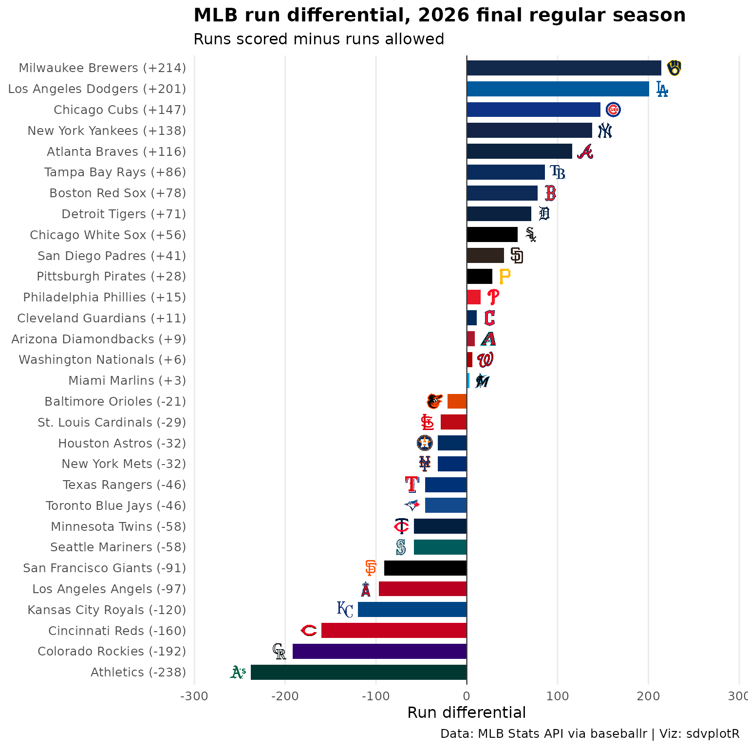
2. Run differential
Every club’s run differential as a bar in its primary color, best at the top, with its logo at the end of the bar.
if (available) {
  rd <- standings |>
    arrange(diff, desc(team_name)) |> # the name breaks a tie, so an unchanged week renders the same
    mutate(
      label = sprintf("%s (%+d)", team_name, diff),
      label = factor(label, levels = label),
      end = diff + sign(diff) * 0.06 * reach
    )

  ggplot(rd, aes(y = label)) +
    geom_col(aes(x = diff, fill = abbreviation), width = 0.72) +
    geom_vline(xintercept = 0, colour = "grey20", linewidth = 0.4) +
    geom_sdv_logos(aes(x = end, team = abbreviation), league = "mlb", height = 0.028) +
    scale_fill_sdv(league = "mlb", guide = "none") +
    scale_x_continuous(limits = c(-1.15, 1.15) * reach) +
    labs(
      title = paste("MLB run differential,", season, through),
      subtitle = "Runs scored minus runs allowed",
      x = "Run differential", y = NULL,
      caption = "Data: MLB Stats API via baseballr | Viz: sdvplotR"
    ) +
    theme_minimal(base_size = 12) +
    theme(
      plot.title = element_text(face = "bold"),
      panel.grid.major.y = element_blank(),
      panel.grid.minor = element_blank()
    )
} else {
  # the Stats API did not answer: a stand-in keeps this figure, which the gallery shows
  ggplot() +
    annotate("text", x = 0, y = 0, size = 5, label = paste0(
      "MLB standings were unavailable when this page was built on ", today, ".\nThey return next week."
    )) +
    theme_void()
}
3. League leaders with headshots
The Stats API’s leaderboards, one category at a time
(mlb_stats_leaders(); the rate stats list qualified players
only). Its player ids are MLBAM ids, which
gt_sdv_headshots(id_system = "league") turns into MLB’s own
headshots. Ties share a rank, so a category can show more than three
players.
categories <- tibble::tribble(
  ~category, ~stat, ~group, ~digits,
  "Home runs", "homeRuns", "hitting", 0,
  "Batting average", "battingAverage", "hitting", 3,
  "OPS", "onBasePlusSlugging", "hitting", 3,
  "Stolen bases", "stolenBases", "hitting", 0,
  "ERA", "earnedRunAverage", "pitching", 2,
  "Strikeouts", "strikeouts", "pitching", 0
)
top3 <- function(i) {
  x <- live(baseballr::mlb_stats_leaders(
    leader_categories = categories$stat[i], season = season, sport_id = 1,
    leader_game_types = "R", limit = 3
  ))
  if (NROW(x) == 0) {
    return(NULL) # the API did not answer for this category
  }
  x |>
    filter(stat_group == categories$group[i], rank <= 3) |>
    transmute(
      category = categories$category[i], rank, person_id, player = person_full_name, team_id,
      value = formatC(as.numeric(value), format = "f", digits = categories$digits[i])
    )
}
leaders <- bind_rows(lapply(seq_len(nrow(categories)), top3))
leaders_ok <- nrow(leaders) > 0
if (leaders_ok) {
  leaders <- leaders |>
    left_join(select(clubs, team_id, abbreviation), by = "team_id") |>
    mutate(
      value = sub("^0\\.", ".", value), # .312, not 0.312, as baseball writes it
      headshot = person_id
    )
}
head(leaders)
#> # A tibble: 6 × 8
#>   category         rank person_id player     team_id value abbreviation headshot
#>   <chr>           <int>     <int> <chr>        <int> <chr> <chr>           <int>
#> 1 Home runs           1    691718 Pete Crow…     112 45    CHC            691718
#> 2 Home runs           1    656941 Kyle Schw…     143 45    PHI            656941
#> 3 Home runs           3    624413 Pete Alon…     110 43    BAL            624413
#> 4 Batting average     1    670541 Yordan Al…     117 .316  HOU            670541
#> 5 Batting average     2    672515 Gabriel M…     109 .311  AZ             672515
#> 6 Batting average     3    650333 Luis Arra…     143 .310  PHI            650333
leaders |>
  select(category, rank, headshot, player, abbreviation, value) |>
  gt(groupname_col = "category", id = "mlb-leaders") |>
  tab_header(
    title = paste("MLB leaders,", season),
    subtitle = paste0("Top three, ", through)
  ) |>
  cols_label(rank = "", headshot = "", player = "Player", abbreviation = "", value = "") |>
  cols_align("right", value) |>
  tab_source_note("Data: MLB Stats API via baseballr | Viz: sdvplotR") |>
  gt_sdv_headshots(columns = headshot, league = "mlb", id_system = "league", height = 36) |>
  gt_sdv_logos(columns = abbreviation, league = "mlb", height = 22) |>
gt_theme_savant()| MLB leaders, 2026 | ||||
| Top three, final regular season | ||||
| Player | ||||
|---|---|---|---|---|
| Home runs | ||||
| 1 |  |
Pete Crow-Armstrong | |
45 |
| 1 |  |
Kyle Schwarber | |
45 |
| 3 |  |
Pete Alonso | |
43 |
| Batting average | ||||
| 1 |  |
Yordan Alvarez | |
.316 |
| 2 |  |
Gabriel Moreno | |
.311 |
| 3 |  |
Luis Arraez | |
.310 |
| OPS | ||||
| 1 | |
Yordan Alvarez | |
1.033 |
| 2 | |
Pete Crow-Armstrong | |
.942 |
| 3 |  |
Willson Contreras | |
.902 |
| Stolen bases | ||||
| 1 |  |
Nasim Nuñez | |
49 |
| 2 |  |
Chandler Simpson | |
46 |
| 3 |  |
Bobby Witt Jr. | |
45 |
| ERA | ||||
| 1 |  |
Jacob Misiorowski | |
1.80 |
| 2 |  |
Cam Schlittler | |
1.95 |
| 3 |  |
Chris Sale | |
2.16 |
| Strikeouts | ||||
| 1 | |
Jacob Misiorowski | |
252 |
| 2 |  |
Gavin Williams | |
248 |
| 3 |  |
Dylan Cease | |
239 |
| 3 | |
Cam Schlittler | |
239 |
| Data: MLB Stats API via baseballr | Viz: sdvplotR | ||||
4. Interactive version
The 30 clubs from the standings in one reactable: click a column
header to sort the league by it (run differential, runs scored, streak),
or search for a club or a division. reactable_sdv_logos()
draws the logos, and reactable_sdv_team_color_bar() fills
each club’s wins cell in its color, to the length of its win total.
league_table <- standings |>
  arrange(desc(pct), team_name) |>
  transmute(logo = abbreviation, team_name, division, w, l, pct, rs, ra, diff, streak)

reactable::reactable(
  league_table,
  searchable = TRUE, highlight = TRUE, compact = TRUE, defaultPageSize = 15,
  columns = list(
    logo = reactable::colDef(name = "", cell = reactable_sdv_logos("mlb", height = 24), html = TRUE, width = 46),
    team_name = reactable::colDef(name = "Team", minWidth = 150),
    division = reactable::colDef(name = "Division", minWidth = 120),
    w = reactable::colDef(name = "W", style = reactable_sdv_team_color_bar(league_table, "logo", "mlb")),
    l = reactable::colDef(name = "L"),
    pct = reactable::colDef(name = "Pct", format = reactable::colFormat(digits = 3)),
    rs = reactable::colDef(name = "RS"),
    ra = reactable::colDef(name = "RA"),
    diff = reactable::colDef(name = "Diff"),
    streak = reactable::colDef(name = "Streak", sortable = FALSE)
  )
)
More recipes like this one, in plotly, ggiraph, leaflet and reactable, are in Interactive charts.
Related
- MLB walks through baseballr and sdvplotR more broadly.
- NHL builds the same three views for hockey.
- Social graphics, automated posts leaderboards like these on a schedule.






Related SportsDataverse packages
- sdvplot - the Python plotting package
- sdvplot-js - the JavaScript / TypeScript plotting packages
- cfbfastR - college football
- hoopR - men’s basketball
- wehoop - women’s basketball
- baseballr - baseball
- fastRhockey - hockey
- oddsapiR - betting odds
- sportyR - playing surfaces
- sportsdataverse-py - the Python package
- sportsdataverse-R - the R meta-package