College Football Weekly Leaderboard

On this page

Updated 2026-10-12: the 2026 season through week 6.

This page is rebuilt every week with the site. It rates every FBS team by opponent-adjusted EPA per play, a simple cousin of SP+ built from the play-by-play, for the latest season with data: the season to date during the fall, the final season in the offseason. Data: cfbfastR play-by-play and CollegeFootballData.com schedules.

Picking the season

Week 0 is in late August, so before then the calendar points at last season. cfbfastR::load_cfb_pbp() errors for a season past its most recent one and warns, returning no rows, for a season whose file is not up yet; either way the page steps back one season. The schedule says whether regular-season games are left, which is what the status line reports. It is a live API call, so it goes through live(): if CollegeFootballData.com does not answer, the page still rates every team from the play-by-play and leaves the records blank for that week instead of failing the site build.

library(sdvplotR)
library(dplyr, warn.conflicts = FALSE)
library(ggplot2)
library(gt)

today <- Sys.Date()
# Week 0 is in late August, so before then the calendar points at last season
current <- as.integer(format(today, "%Y")) - (format(today, "%m") < "08")

# A season's play-by-play, or NULL when it is not published: load_cfb_pbp() errors
# for a season past cfbfastR's most recent one, and warns and returns no rows for
# one whose file is not up yet
play_by_play <- function(season) {
  pbp <- tryCatch(suppressWarnings(cfbfastR::load_cfb_pbp(season)), error = function(e) NULL)
  if (NROW(pbp) == 0) NULL else pbp
}

season <- current
pbp <- play_by_play(season)
if (is.null(pbp)) {
  season <- current - 1
  pbp <- play_by_play(season)
}
stopifnot(!is.null(pbp))

# A live API call, or NULL when the API does not answer: one bad week then shows
# a note instead of failing the whole site build
live <- function(expr) tryCatch(expr, error = function(e) NULL)

# CollegeFootballData.com's schedule (a live API: set CFBD_API_KEY, a free key)
schedule <- live(cfbfastR::load_cfb_schedules(season))
schedule_ok <- NROW(schedule) > 0
if (schedule_ok) {
  played <- schedule |>
    filter(completed) |>
    arrange(start_date, game_id)
  week <- max(played$week[played$season_type == "regular"])
  left <- filter(schedule, !completed)
} else {
  week <- max(pbp$week)
}
if (!schedule_ok) {
  status <- sprintf(
    "the %d season through week %d. CollegeFootballData.com's schedule was unavailable when this page was built, so records are missing this week; they return next week.",
    season, week
  )
  through <- paste("through week", week)
} else if (any(left$season_type == "regular")) {
  status <- sprintf("the %d season through week %d.", season, week)
  through <- paste("through week", week)
} else if (nrow(left) > 0) {
  status <- sprintf("the %d regular season is final; bowls and the playoff are under way.", season)
  through <- "regular season and finished bowls"
} else {
  status <- sprintf("the offseason, so this is the final %d season, bowls and playoff included.", season)
  through <- "final"
}

The play-by-play carries each game’s teams with their division and conference, which picks out the FBS teams. Records come from the schedule’s played games, against FBS and FCS opponents alike.

sides <- bind_rows(
  distinct(pbp, game_id, week, school = home, conference = home_team_conference, division = home_team_division),
  distinct(pbp, game_id, week, school = away, conference = away_team_conference, division = away_team_division)
)
fbs <- sides |>
  filter(division %in% "fbs") |>
  arrange(week, game_id) |>
  group_by(school) |>
  summarise(conference = last(conference), .groups = "drop") |>
  # the index keys three conferences by their short codes
  mutate(conference = recode(conference, "American Athletic" = "AAC", "Conference USA" = "CUSA", "FBS Independents" = "FBS Indep."))

if (schedule_ok) {
  records <- bind_rows(
    transmute(played, school = home_team, win = home_points > away_points),
    transmute(played, school = away_team, win = away_points > home_points)
  ) |>
    group_by(school) |>
    summarise(record = paste(sum(win), sum(!win), sep = "-"), .groups = "drop")
  fbs <- left_join(fbs, records, by = "school")
} else {
  fbs$record <- NA_character_ # shown as a dash
}
nrow(fbs)
#> [1] 138

1. Top 25 by adjusted EPA per play

The ratings use FBS-against-FBS pass and run plays, minus garbage time (a lead of more than 43 points in the first quarter, 37 in the second, 27 in the third or 21 in the fourth). One pass of opponent adjustment credits each offensive play for the defense it faced (that defense’s EPA allowed per play against the FBS average), and each defensive play for the offense it faced. Net is adjusted offense minus adjusted defense.

plays <- pbp |>
  filter(
    pass == 1 | rush == 1, !is.na(EPA),
    pos_team %in% fbs$school, def_pos_team %in% fbs$school
  ) |>
  mutate(margin = c(43, 37, 27, 21)[period]) |> # NA in overtime, which is never garbage time
  filter(!coalesce(abs(pos_score_diff_start) > margin, FALSE)) |>
  arrange(game_id, id_play) # a fixed order, so every mean sums the same way each week

avg <- mean(plays$EPA)
defense_allows <- plays |>
  group_by(def_pos_team) |>
  summarise(allowed = mean(EPA), .groups = "drop")
offense_gains <- plays |>
  group_by(pos_team) |>
  summarise(gained = mean(EPA), .groups = "drop")
adjusted <- plays |>
  left_join(defense_allows, by = "def_pos_team") |>
  left_join(offense_gains, by = "pos_team") |>
  mutate(adj_off = EPA - (allowed - avg), adj_def = EPA - (gained - avg))

ratings <- inner_join(
  adjusted |> group_by(school = pos_team) |> summarise(off = mean(adj_off), .groups = "drop"),
  adjusted |> group_by(school = def_pos_team) |> summarise(dfn = mean(adj_def), .groups = "drop"),
  by = "school"
) |>
  mutate(net = off - dfn) |>
  inner_join(fbs, by = "school") |>
  # "Charlotte" alone is the 49ers or the Saints; the 49ers are the FBS team
  mutate(key = sub("^Charlotte$", "Charlotte 49ers", school)) |>
  arrange(desc(net), school) |> # the school breaks a tie, so an unchanged week renders the same
  mutate(rank = row_number())

top25 <- ratings |>
  slice_head(n = 25) |>
  mutate(logo = key, conf_logo = conference) |>
  select(rank, logo, school, conf_logo, conference, record, off, dfn, net)
head(top25)
#> # A tibble: 6 × 9
#>    rank logo       school     conf_logo  conference record   off     dfn   net
#>   <int> <chr>      <chr>      <chr>      <chr>      <chr>  <dbl>   <dbl> <dbl>
#> 1     1 Alabama    Alabama    SEC        SEC        5-1    0.307 -0.0764 0.383
#> 2     2 Georgia    Georgia    SEC        SEC        6-0    0.276 -0.108  0.383
#> 3     3 Notre Dame Notre Dame FBS Indep. FBS Indep. 6-0    0.257 -0.125  0.382
#> 4     4 Wisconsin  Wisconsin  Big Ten    Big Ten    4-1    0.170 -0.188  0.357
#> 5     5 Indiana    Indiana    Big Ten    Big Ten    6-0    0.240 -0.110  0.350
#> 6     6 Nebraska   Nebraska   Big Ten    Big Ten    5-1    0.205 -0.123  0.327

sdvplotR has a row for every FBS conference too, so gt_sdv_logos() draws the conference marks from the play-by-play’s conference names, next to the school logos.

top25 |>
  gt(id = "cfb-top25") |>
  tab_header(
    title = paste("College football top 25,", season),
    subtitle = paste("Opponent-adjusted EPA per play,", through)
  ) |>
  fmt_number(c(off, dfn, net), decimals = 3, force_sign = TRUE) |>
  sub_missing(record, missing_text = "—") |>
  data_color(net, palette = c("#f7f7f7", "#2e8b57"), domain = c(0, max(top25$net))) |>
  tab_spanner("Adjusted EPA per play", c(off, dfn, net)) |>
  cols_label(
    rank = "", logo = "", school = "Team", conf_logo = "", conference = "Conference",
    record = "Record", off = "Offense", dfn = "Defense", net = "Net"
  ) |>
  tab_source_note(paste(
    "Data: cfbfastR play-by-play and CollegeFootballData.com schedules.",
    "FBS vs FBS pass and run plays, garbage time removed; defense is EPA allowed",
    "(lower is better). Viz: sdvplotR"
  )) |>
  gt_sdv_logos(columns = logo, league = "cfb", height = 26) |>
  gt_sdv_logos(columns = conf_logo, league = "cfb", height = 20) |>
  gt_theme_ncaa()

toss_out_spanner_dev
College football top 25, 2026
Opponent-adjusted EPA per play, through week 6
	Team	Conference	Record	Adjusted EPA per play
	Team	Conference	Record	Offense	Defense	Net
1	Alabama	SEC	5-1	+0.307	−0.076	+0.383
2	Georgia	SEC	6-0	+0.276	−0.108	+0.383
3	Notre Dame	FBS Indep.	6-0	+0.257	−0.125	+0.382
4	Wisconsin	Big Ten	4-1	+0.170	−0.188	+0.357
5	Indiana	Big Ten	6-0	+0.240	−0.110	+0.350
6	Nebraska	Big Ten	5-1	+0.205	−0.123	+0.327
7	LSU	SEC	4-2	+0.088	−0.211	+0.299
8	Miami	ACC	5-0	+0.274	−0.004	+0.278
9	Ohio State	Big Ten	5-1	+0.213	−0.049	+0.262
10	Texas	SEC	4-1	+0.104	−0.157	+0.261
11	Missouri	SEC	5-1	+0.115	−0.138	+0.253
12	Mississippi State	SEC	4-1	+0.242	−0.001	+0.242
13	Utah	Big 12	5-0	+0.254	+0.012	+0.242
14	BYU	Big 12	5-0	+0.136	−0.101	+0.237
15	Northwestern	Big Ten	4-1	+0.280	+0.051	+0.230
16	Wake Forest	ACC	5-1	+0.159	−0.061	+0.220
17	Oregon	Big Ten	3-2	+0.071	−0.125	+0.197
18	Kansas	Big 12	2-3	+0.165	−0.028	+0.193
19	Oklahoma	SEC	3-2	+0.079	−0.111	+0.190
20	Louisville	ACC	3-3	+0.191	+0.027	+0.165
21	UCLA	Big Ten	5-0	+0.115	−0.043	+0.158
22	Liberty	CUSA	5-1	+0.158	+0.012	+0.145
23	Michigan	Big Ten	3-2	+0.110	−0.034	+0.145
24	Arizona	Big 12	5-1	+0.192	+0.060	+0.132
25	USC	Big Ten	6-1	+0.309	+0.178	+0.130
Data: cfbfastR play-by-play and CollegeFootballData.com schedules. FBS vs FBS pass and run plays, garbage time removed; defense is EPA allowed (lower is better). Viz: sdvplotR

2. Every FBS team, by conference

One row per conference, ordered by its average rating, each team’s logo at its net rating (nudged up and down in turn so neighbors overlap less). The bar in the conference’s color spans it from its lowest team to its highest, and the tick marks its average. The colors come from sdv_teams(include_conferences = TRUE) and scale_y_sdv() draws the conference marks on the axis from the conference keys (theme_y_sdv() lets the axis draw images).

conf_order <- ratings |>
  group_by(conference) |>
  summarise(mean_net = mean(net), lo = min(net), hi = max(net), .groups = "drop") |>
  arrange(mean_net, conference) |>
  mutate(row = row_number(), conference = factor(conference, levels = conference))
teams <- ratings |>
  inner_join(select(conf_order, conference, row) |> mutate(conference = as.character(conference)), by = "conference") |>
  arrange(row, net, school) |>
  group_by(conference) |>
  mutate(y = row + if_else(row_number() %% 2 == 0, 0.17, -0.17)) |>
  ungroup()

conf_rows <- sdv_teams("cfb", include_conferences = TRUE) |>
  filter(program == "conference")
conf_colors <- setNames(conf_rows$color_primary, conf_rows$team_id)

ggplot() +
  geom_vline(xintercept = 0, linetype = "dashed", colour = "grey60") +
  geom_segment(
    data = conf_order,
    aes(x = lo, xend = hi, y = conference, yend = conference, colour = conference),
    linewidth = 7, alpha = 0.35, lineend = "round"
  ) +
  geom_point(
    data = conf_order, aes(x = mean_net, y = conference, colour = conference),
    shape = "|", size = 9
  ) +
  # a discrete axis still takes numbers: row 3 is the third conference, so 3.17 sits just above it
  geom_sdv_logos(data = teams, aes(x = net, y = y, team = key), league = "cfb", height = 0.04) +
  scale_colour_manual(values = conf_colors, guide = "none") +
  scale_y_sdv(league = "cfb", size = 30, expand = expansion(add = 0.6)) +
  scale_x_continuous(expand = expansion(mult = 0.04)) +
  labs(
    title = paste("FBS teams by conference,", season, through),
    subtitle = "Net opponent-adjusted EPA per play; the tick marks the conference average",
    x = "Net adjusted EPA per play", y = NULL,
    caption = "Data: cfbfastR | Viz: sdvplotR"
  ) +
  theme_minimal(base_size = 13) +
  theme(
    plot.title = element_text(face = "bold"),
    panel.grid.minor = element_blank(),
    panel.grid.major.y = element_blank()
  ) +
  theme_y_sdv()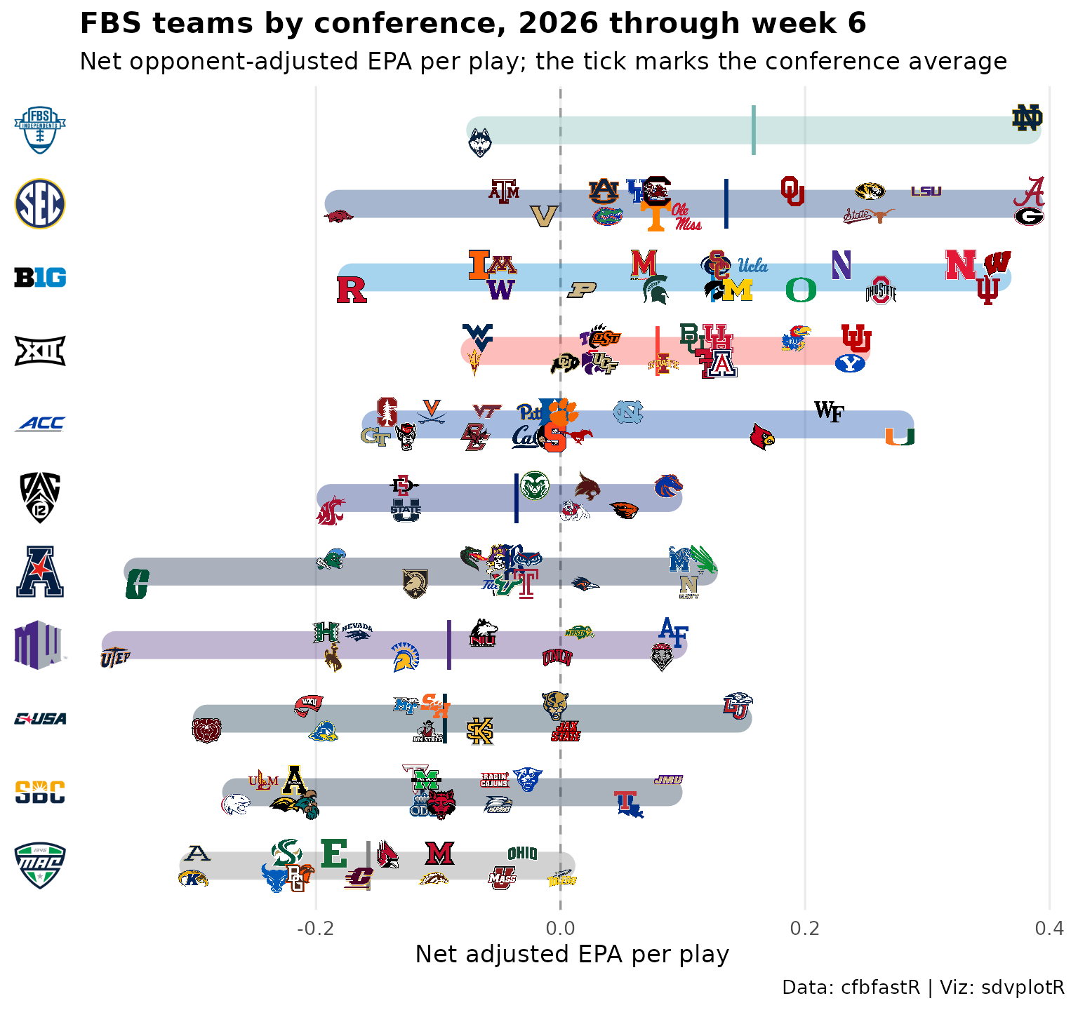

Every FBS team's logo placed by its net opponent-adjusted EPA per play, one row per conference ordered by average rating, with each conference's logo on the vertical axis and a bar in its color spanning its teams.

3. Offense and defense of the top 25

The two halves of the rating for the top 25, one logo each. The defense axis is reversed so the better defenses sit higher, and the dashed lines are the top 25’s averages.

ggplot(top25, aes(x = off, y = dfn)) +
  geom_hline(yintercept = mean(top25$dfn), linetype = "dashed", colour = "grey55") +
  geom_vline(xintercept = mean(top25$off), linetype = "dashed", colour = "grey55") +
  geom_sdv_logos(aes(team = logo), league = "cfb", height = 0.075) +
  scale_x_continuous(expand = expansion(mult = 0.08)) +
  scale_y_reverse(expand = expansion(mult = 0.08)) +
  labs(
    title = paste("How the top 25 get there,", season),
    subtitle = paste("Opponent-adjusted EPA per play,", through),
    x = "Adjusted offense: EPA per play",
    y = "Adjusted defense: EPA allowed per play (reversed)",
    caption = "Data: cfbfastR | Viz: sdvplotR"
  ) +
  theme_minimal(base_size = 13) +
  theme(plot.title = element_text(face = "bold"), panel.grid.minor = element_blank())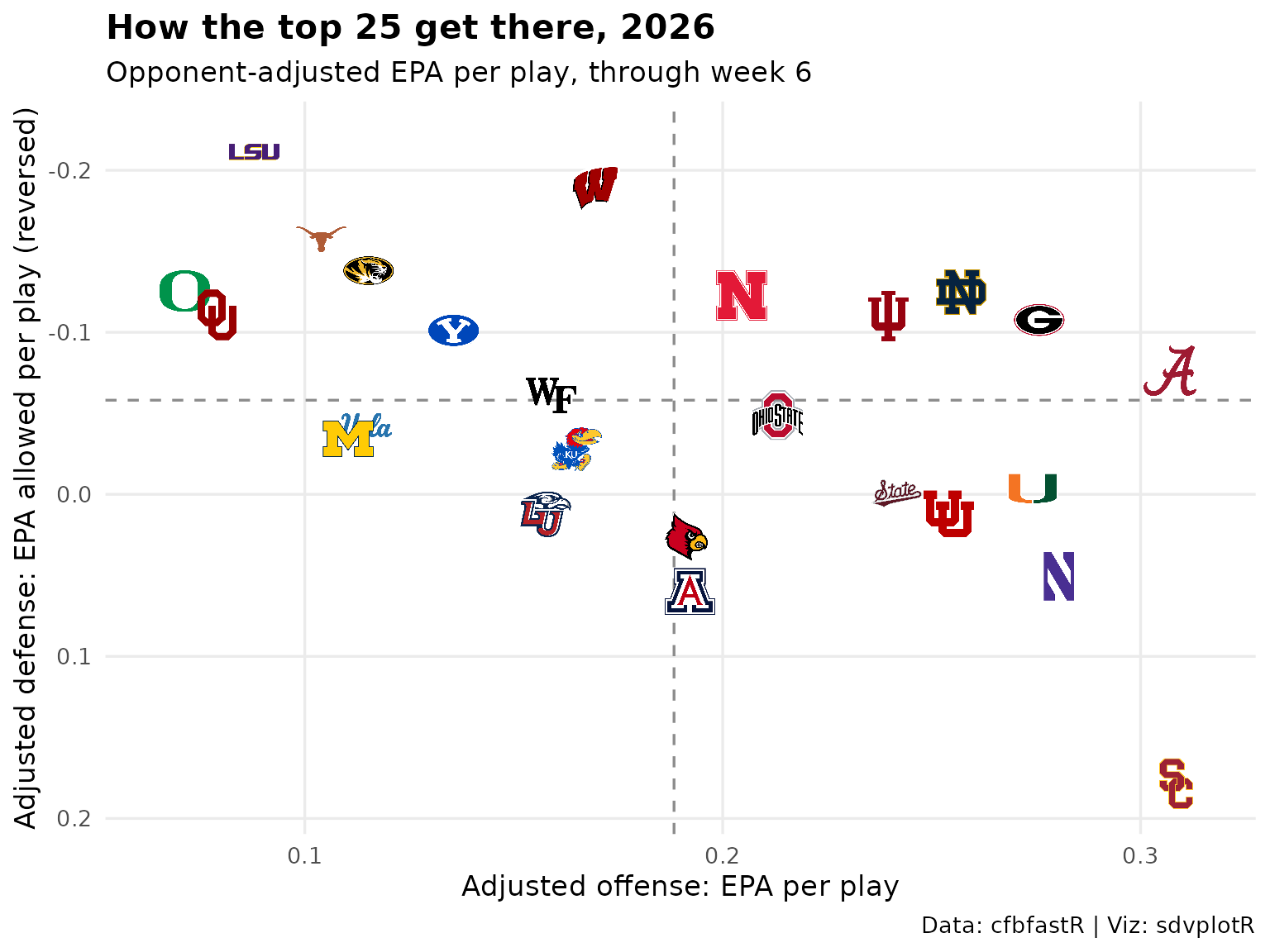

The top 25 college football teams' logos placed by adjusted offensive EPA per play (horizontal) and adjusted defensive EPA allowed per play (vertical, reversed so better defenses sit higher), with dashed lines at the group's averages.

4. Interactive version

The top 25 table stops at 25. Every FBS team’s rating goes in a reactable instead, which sorts on any column header and searches in the browser: type a school or a conference to find it. reactable_sdv_logos() draws the school and conference marks from the same keys as gt_sdv_logos() above.

every_team <- ratings |>
  transmute(rank, logo = key, school, conf_logo = conference, conference, record, off, dfn, net)
logo_col <- function(height) {
  reactable::colDef(name = "", cell = reactable_sdv_logos("cfb", height = height), html = TRUE, width = 46, sortable = FALSE)
}
epa_col <- function(name) reactable::colDef(name = name, format = reactable::colFormat(digits = 3))

reactable::reactable(
  every_team,
  searchable = TRUE, highlight = TRUE, compact = TRUE, defaultPageSize = 15,
  columns = list(
    rank = reactable::colDef(name = "", width = 46),
    logo = logo_col(26),
    school = reactable::colDef(name = "Team", minWidth = 130),
    conf_logo = logo_col(20),
    conference = reactable::colDef(name = "Conference", minWidth = 110),
    record = reactable::colDef(name = "Record", na = "—"),
    off = epa_col("Offense"),
    dfn = epa_col("Defense"),
    net = epa_col("Net")
  )
)

More recipes like this one, in plotly, ggiraph, leaflet and reactable, are in Interactive charts.

NFL weekly runs the same EPA tables on nflverse data.
College Football walks through cfbfastR and sdvplotR more broadly.
Social graphics, automated posts tables like these on a schedule.

Our Authors

Citation

To cite the sdvplotR R package in publications, use:

BibTeX Citation

@misc{gilani_carl_lee_kay_weatherman_sdvplotR,
  author = {Gilani, Saiem and Carl, Sebastian and Lee, Jared and Kay, Camden and Weatherman, Andrew},
  title = {sdvplotR: The SportsDataverse's R Package for Multi-League Sports Plotting.},
  url = {https://sdvplotR.sportsdataverse.org},
  year = {2026}
}

sdvplot - the Python plotting package
sdvplot-js - the JavaScript / TypeScript plotting packages
cfbfastR - college football
hoopR - men’s basketball
wehoop - women’s basketball
baseballr - baseball
fastRhockey - hockey
oddsapiR - betting odds
sportyR - playing surfaces
sportsdataverse-py - the Python package
sportsdataverse-R - the R meta-package

Saiem Gilani