NFL Weekly Leaderboard

On this page

Updated 2026-10-12: the 2026 season through week 5 (78 games).

This page is rebuilt every week with the site. It finds the latest NFL season with play-by-play, ranks every team by EPA (expected points added) per play, plots offense against defense, and lists the most efficient quarterbacks with their headshots: the season to date while games are being played, the last full regular season in the offseason. Data: nflverse play-by-play and schedules, read with nflreadr.

Picking the season

The season starts in September, so before then the calendar points at last season. nflverse publishes a season’s play-by-play file with its first games; until then nflreadr::load_pbp() errors, and the page steps back one season instead of failing. The status line above comes from the schedule: games still to play mean the season to date, a played Super Bowl means the offseason.

library(sdvplotR)
library(dplyr, warn.conflicts = FALSE)
library(ggplot2)
library(gt)

today <- Sys.Date()
# The season starts in September, so before then the calendar points at last season
current <- as.integer(format(today, "%Y")) - (format(today, "%m") < "09")

# A season's regular-season plays, or NULL when nflverse has not published any:
# load_pbp() errors for a season past nflreadr::most_recent_season()
regular_season <- function(season) {
  pbp <- tryCatch(nflreadr::load_pbp(season), error = function(e) NULL)
  if (is.null(pbp)) {
    return(NULL)
  }
  pbp <- filter(pbp, season_type == "REG")
  if (nrow(pbp) == 0) NULL else pbp
}

season <- current
pbp <- regular_season(season)
if (is.null(pbp)) {
  season <- current - 1
  pbp <- regular_season(season)
}
stopifnot(!is.null(pbp))

schedule <- nflreadr::load_schedules(season)
week <- max(pbp$week)
n_games <- n_distinct(pbp$game_id)
unplayed <- sum(schedule$game_type == "REG" & is.na(schedule$result))
super_bowl <- any(schedule$game_type == "SB" & !is.na(schedule$result))
through <- if (unplayed > 0) paste("through week", week) else "final regular season"
status <- if (unplayed > 0) {
  sprintf("the %d season through week %d (%d games).", season, week, n_games)
} else if (!super_bowl) {
  sprintf("the final %d regular season; the playoffs are under way.", season)
} else {
  sprintf(
    "the offseason, so this is the final %d regular season. The %d season starts in September.",
    season, season + 1
  )
}

1. Power table

Every team’s record and point differential from the schedule, and its EPA per pass or run play on offense and allowed on defense, from the play-by-play. Net EPA per play is offense minus defense; the trend compares each team’s last three games with its season. gt_merge_stack_team_color() stacks the record under the nickname in team colors, gt_delta() computes the trend, and gt_sdv_logos() turns the nflverse abbreviations into logos.

plays <- pbp |>
  filter(pass == 1 | rush == 1, !is.na(epa), !is.na(posteam))
offense <- plays |>
  group_by(game_id, week, team = posteam) |>
  summarise(off = sum(epa), off_n = n(), .groups = "drop")
defense <- plays |>
  group_by(game_id, team = defteam) |>
  summarise(dfn = sum(epa), dfn_n = n(), .groups = "drop")
# a fixed row order: every sum below adds up in the same order each week
per_game <- inner_join(offense, defense, by = c("game_id", "team")) |>
  arrange(team, week)

per_play <- function(games) {
  games |>
    group_by(team) |>
    summarise(
      off_epa = sum(off) / sum(off_n),
      def_epa = sum(dfn) / sum(dfn_n),
      .groups = "drop"
    ) |>
    mutate(net = off_epa - def_epa)
}
last3 <- per_game |>
  group_by(team) |>
  slice_tail(n = 3) |>
  ungroup() |>
  per_play() |>
  select(team, last3 = net)

games <- filter(schedule, game_type == "REG", game_id %in% pbp$game_id)
record <- bind_rows(
  transmute(games, team = home_team, pf = home_score, pa = away_score),
  transmute(games, team = away_team, pf = away_score, pa = home_score)
) |>
  group_by(team) |>
  summarise(
    w = sum(pf > pa), l = sum(pf < pa), t = sum(pf == pa), diff = sum(pf - pa),
    .groups = "drop"
  ) |>
  mutate(record = if_else(t > 0, paste(w, l, t, sep = "-"), paste(w, l, sep = "-")))

nicknames <- nflreadr::load_teams() |>
  select(team = team_abbr, name = team_nick)

power <- per_play(per_game) |>
  inner_join(last3, by = "team") |>
  inner_join(record, by = "team") |>
  inner_join(nicknames, by = "team") |>
  arrange(desc(net), team) |> # the team breaks a tie, so an unchanged week renders the same
  mutate(rank = row_number()) |>
  select(rank, team, name, record, diff, off_epa, def_epa, net, last3)
head(power)
#> # A tibble: 6 × 9
#>    rank team  name    record  diff  off_epa  def_epa   net  last3
#>   <int> <chr> <chr>   <chr>  <int>    <dbl>    <dbl> <dbl>  <dbl>
#> 1     1 SF    49ers   5-0       61  0.187   -0.0723  0.260 0.176 
#> 2     2 KC    Chiefs  4-0       41  0.157   -0.0314  0.188 0.122 
#> 3     3 JAX   Jaguars 4-1       53  0.105   -0.0732  0.178 0.194 
#> 4     4 MIN   Vikings 5-0       45 -0.0999  -0.235   0.135 0.145 
#> 5     5 BAL   Ravens  4-1       27  0.132    0.00232 0.129 0.0973
#> 6     6 LA    Rams    2-2        2  0.00599 -0.0977  0.104 0.266

good_bad <- c("#c84630", "#f7f7f7", "#2e8b57")
reach <- max(abs(c(power$off_epa, power$def_epa))) # one symmetric scale for both sides

power |>
  gt(id = "nfl-power") |> # a fixed id: gt draws a random one otherwise
  tab_header(
    title = paste("NFL power table,", season),
    subtitle = paste("Ranked by net EPA per play,", through)
  ) |>
  fmt_number(c(off_epa, def_epa, net, last3), decimals = 3, force_sign = TRUE) |>
  fmt_number(diff, decimals = 0, force_sign = TRUE) |>
  data_color(off_epa, palette = good_bad, domain = c(-reach, reach)) |>
  data_color(def_epa, palette = rev(good_bad), domain = c(-reach, reach)) |>
  data_color(net, palette = good_bad, domain = c(-1, 1) * max(abs(power$net))) |>
  tab_spanner("EPA per play", c(off_epa, def_epa, net, last3)) |>
  cols_label(
    rank = "", team = "", name = "Team", diff = "Pt diff",
    off_epa = "Offense", def_epa = "Defense", net = "Net", last3 = "Last 3"
  ) |>
  tab_source_note(paste(
    "Data: nflverse play-by-play via nflreadr. Pass and run plays;",
    "defense is EPA allowed (lower is better). Viz: sdvplotR"
  )) |>
  gt_merge_stack_team_color(name, record, team, league = "nfl") |>
  gt_delta(net, last3, column_label = "Trend", decimals = 3, arrows = TRUE) |>
  gt_sdv_logos(columns = team, league = "nfl", height = 26) |>
  gt_theme_athletic()

	Team	Pt diff	EPA per play				Trend
NFL power table, 2026
Ranked by net EPA per play, through week 5
	Team	Pt diff	Offense	Defense	Net	Last 3	Trend
1	49ers 5-0	+61	+0.187	−0.072	+0.260	+0.176	▼ 0.083
2	Chiefs 4-0	+41	+0.157	−0.031	+0.188	+0.122	▼ 0.066
3	Jaguars 4-1	+53	+0.105	−0.073	+0.178	+0.194	▲ 0.016
4	Vikings 5-0	+45	−0.100	−0.235	+0.135	+0.145	▲ 0.010
5	Ravens 4-1	+27	+0.132	+0.002	+0.129	+0.097	▼ 0.032
6	Rams 2-2	+2	+0.006	−0.098	+0.104	+0.266	▲ 0.162
7	Bengals 3-2	+19	+0.068	−0.023	+0.091	+0.054	▼ 0.037
8	Bills 3-1	+20	+0.195	+0.117	+0.078	+0.037	▼ 0.041
9	Panthers 2-2	+12	+0.086	+0.016	+0.070	+0.180	▲ 0.110
10	Patriots 3-2	+16	+0.048	−0.015	+0.064	+0.027	▼ 0.036
11	Seahawks 3-2	+29	−0.070	−0.113	+0.043	−0.099	▼ 0.142
12	Bears 3-2	+23	+0.038	+0.004	+0.034	+0.016	▼ 0.018
13	Raiders 3-2	+3	+0.019	−0.015	+0.033	−0.072	▼ 0.106
14	Texans 1-4	−2	+0.003	−0.016	+0.019	+0.151	▲ 0.132
15	Falcons 2-3	−3	−0.024	−0.035	+0.011	+0.242	▲ 0.231
16	Jets 2-3	−3	−0.024	−0.035	+0.010	−0.073	▼ 0.083
17	Lions 3-2	+16	+0.176	+0.166	+0.010	+0.084	▲ 0.074
18	Packers 3-2	−8	−0.013	−0.009	−0.004	+0.096	▲ 0.101
19	Broncos 3-2	−14	−0.054	−0.035	−0.019	+0.052	▲ 0.071
20	Steelers 3-2	+2	−0.023	−0.002	−0.021	+0.046	▲ 0.067
21	Cowboys 2-3	+2	+0.157	+0.182	−0.024	−0.068	▼ 0.043
22	Buccaneers 1-4	−12	−0.092	−0.059	−0.034	+0.044	▲ 0.077
23	Browns 3-2	−19	−0.063	−0.022	−0.041	+0.002	▲ 0.043
24	Giants 3-1-1	+3	−0.007	+0.048	−0.055	+0.063	▲ 0.118
25	Commanders 1-3-1	−34	−0.008	+0.050	−0.058	−0.057	▲ 0.001
26	Colts 2-3	−14	−0.038	+0.067	−0.105	−0.024	▲ 0.082
27	Saints 1-4	−33	−0.040	+0.089	−0.129	−0.261	▼ 0.132
28	Chargers 0-5	−45	−0.192	−0.053	−0.139	−0.049	▲ 0.089
29	Cardinals 1-4	−54	−0.013	+0.133	−0.146	−0.218	▼ 0.073
30	Eagles 2-3	−20	−0.111	+0.049	−0.159	−0.267	▼ 0.107
31	Titans 0-5	−51	−0.136	+0.057	−0.193	−0.226	▼ 0.033
32	Dolphins 0-5	−62	−0.118	+0.106	−0.223	−0.193	▲ 0.030
Data: nflverse play-by-play via nflreadr. Pass and run plays; defense is EPA allowed (lower is better). Viz: sdvplotR

gt_save_crop(table, "nfl-power.png") renders the same table to a trimmed PNG, ready to post; see Saving and Posting Tables.

2. Offense against defense

The same EPA per play as a scatter, one logo per team. The y axis is reversed so the better defenses sit higher: the top-right corner is where good teams live. The faint diagonals are lines of equal net EPA per play, 0.1 apart.

ggplot(power, aes(x = off_epa, y = def_epa)) +
  geom_abline(slope = 1, intercept = seq(-0.6, 0.6, by = 0.1), colour = "grey88", linewidth = 0.3) +
  geom_hline(yintercept = mean(power$def_epa), linetype = "dashed", colour = "grey55") +
  geom_vline(xintercept = mean(power$off_epa), linetype = "dashed", colour = "grey55") +
  geom_sdv_logos(aes(team = team), league = "nfl", width = 0.06, alpha = 0.9) +
  # logos do not widen the limits, so leave room for the outermost ones
  scale_x_continuous(expand = expansion(mult = 0.07)) +
  scale_y_reverse(expand = expansion(mult = 0.07)) +
  labs(
    title = paste("NFL offense and defense,", season),
    subtitle = paste("EPA per pass or run play,", through),
    x = "Offense: EPA per play",
    y = "Defense: EPA allowed per play (reversed)",
    caption = "Data: nflverse via nflreadr | Viz: sdvplotR"
  ) +
  theme_minimal(base_size = 13) +
  theme(plot.title = element_text(face = "bold"), panel.grid.minor = element_blank())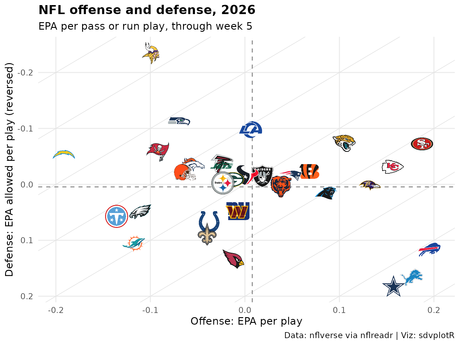

Every NFL team's logo placed by offensive EPA per play (horizontal) and defensive EPA allowed per play (vertical, reversed so better defenses sit higher), with dashed league-average lines and faint diagonals of equal net EPA.

3. Quarterback leaderboard

EPA per dropback (passes, sacks and scrambles) for quarterbacks with at least 15 dropbacks per team game, with completion percentage over expected (CPOE). The play-by-play’s id column is the passer’s GSIS id, which is what gt_sdv_headshots() takes for the NFL; the season’s rosters, keyed by the same id, give the full names.

team_games <- max(count(per_game, team)$n)
qbs <- pbp |>
  filter(qb_dropback == 1, !is.na(qb_epa), !is.na(id)) |>
  arrange(game_id, play_id) |>
  group_by(id) |>
  summarise(
    name = last(name),
    team = last(posteam),
    dropbacks = n(),
    epa = mean(qb_epa),
    cpoe = mean(cpoe, na.rm = TRUE),
    success = mean(success, na.rm = TRUE),
    td = sum(pass_touchdown, na.rm = TRUE),
    int = sum(interception, na.rm = TRUE),
    .groups = "drop"
  ) |>
  filter(dropbacks >= 15 * team_games) |>
  arrange(desc(epa), id) |>
  mutate(rank = row_number(), headshot = id)
full_names <- nflreadr::load_rosters(season) |>
  distinct(id = gsis_id, full_name) |>
  filter(!is.na(id), !duplicated(id))
qbs <- qbs |>
  left_join(full_names, by = "id") |>
  mutate(name = coalesce(full_name, name))
nrow(qbs)
#> [1] 31

qbs |>
  slice_head(n = 16) |>
  select(rank, headshot, name, team, dropbacks, epa, cpoe, success, td, int) |>
  gt(id = "nfl-qbs") |>
  tab_header(
    title = paste("NFL quarterbacks by EPA per dropback,", season),
    subtitle = paste0("Minimum ", 15 * team_games, " dropbacks, ", through)
  ) |>
  fmt_number(epa, decimals = 3, force_sign = TRUE) |>
  fmt_number(cpoe, decimals = 1, force_sign = TRUE) |>
  fmt_percent(success, decimals = 1) |>
  cols_label(
    rank = "", headshot = "", name = "Quarterback", team = "", dropbacks = "Dropbacks",
    epa = "EPA/db", cpoe = "CPOE", success = "Success", td = "TD", int = "INT"
  ) |>
  tab_source_note("Data: nflverse play-by-play via nflreadr | Viz: sdvplotR") |>
  gt_color_pills(
    epa,
    palette = good_bad, domain = c(-1, 1) * max(abs(qbs$epa)), digits = 3, pill_height = 22
  ) |>
  gt_sdv_headshots(columns = headshot, league = "nfl", id_system = "gsis", height = 34) |>
  gt_sdv_logos(columns = team, league = "nfl", height = 22) |>
  gt_theme_sdv()

	Quarterback	Dropbacks	EPA/db	CPOE	Success	TD	INT
NFL quarterbacks by EPA per dropback, 2026
Minimum 75 dropbacks, through week 5
1	Brock Purdy	157	0.417	+4.7	57.3%	13	2
2	Lamar Jackson	111	0.375	+8.1	57.7%	6	1
3	Josh Allen	138	0.318	+6.0	44.2%	6	3
4	Michael Penix Jr.	84	0.311	+1.1	52.4%	3	1
5	Jared Goff	207	0.308	+1.3	50.2%	12	0
6	Trevor Lawrence	158	0.269	+5.9	49.4%	10	3
7	Bryce Young	175	0.254	+5.7	46.3%	9	2
8	Dak Prescott	211	0.217	+1.9	50.2%	9	3
9	Patrick Mahomes	143	0.205	+0.8	49.0%	9	2
10	Drake Maye	180	0.204	+6.7	52.8%	8	7
11	Jayden Daniels	100	0.189	+2.1	45.0%	3	0
12	Kirk Cousins	183	0.186	+1.4	48.6%	12	4
13	Joe Burrow	204	0.173	+6.0	50.0%	11	3
14	C.J. Stroud	202	0.127	+2.5	48.5%	6	0
15	Jordan Love	197	0.111	−3.1	43.1%	10	3
16	Matthew Stafford	169	0.087	−0.1	46.7%	6	6
Data: nflverse play-by-play via nflreadr \| Viz: sdvplotR

The same quarterbacks on the two axes, each drawn as his headshot. Up and to the right is efficient and accurate.

ggplot(qbs, aes(x = cpoe, y = epa)) +
  geom_hline(yintercept = mean(qbs$epa), linetype = "dashed", colour = "grey55") +
  geom_vline(xintercept = mean(qbs$cpoe), linetype = "dashed", colour = "grey55") +
  geom_sdv_headshots(aes(player_id = id), league = "nfl", id_system = "gsis", height = 0.08) +
  ggrepel::geom_text_repel(
    aes(label = sub("^\\S+\\s+", "", name)), # the last name
    size = 3, colour = "grey25", point.size = 13, box.padding = 0.35,
    min.segment.length = 0, segment.colour = "grey70", max.overlaps = Inf,
    seed = 2026 # a seed: the same layout each week
  ) +
  labs(
    title = paste("NFL quarterbacks,", season),
    subtitle = paste0("EPA per dropback against CPOE, minimum ", 15 * team_games, " dropbacks, ", through),
    x = "Completion percentage over expected",
    y = "EPA per dropback",
    caption = "Data: nflverse via nflreadr | Viz: sdvplotR"
  ) +
  theme_minimal(base_size = 13) +
  theme(plot.title = element_text(face = "bold"), panel.grid.minor = element_blank())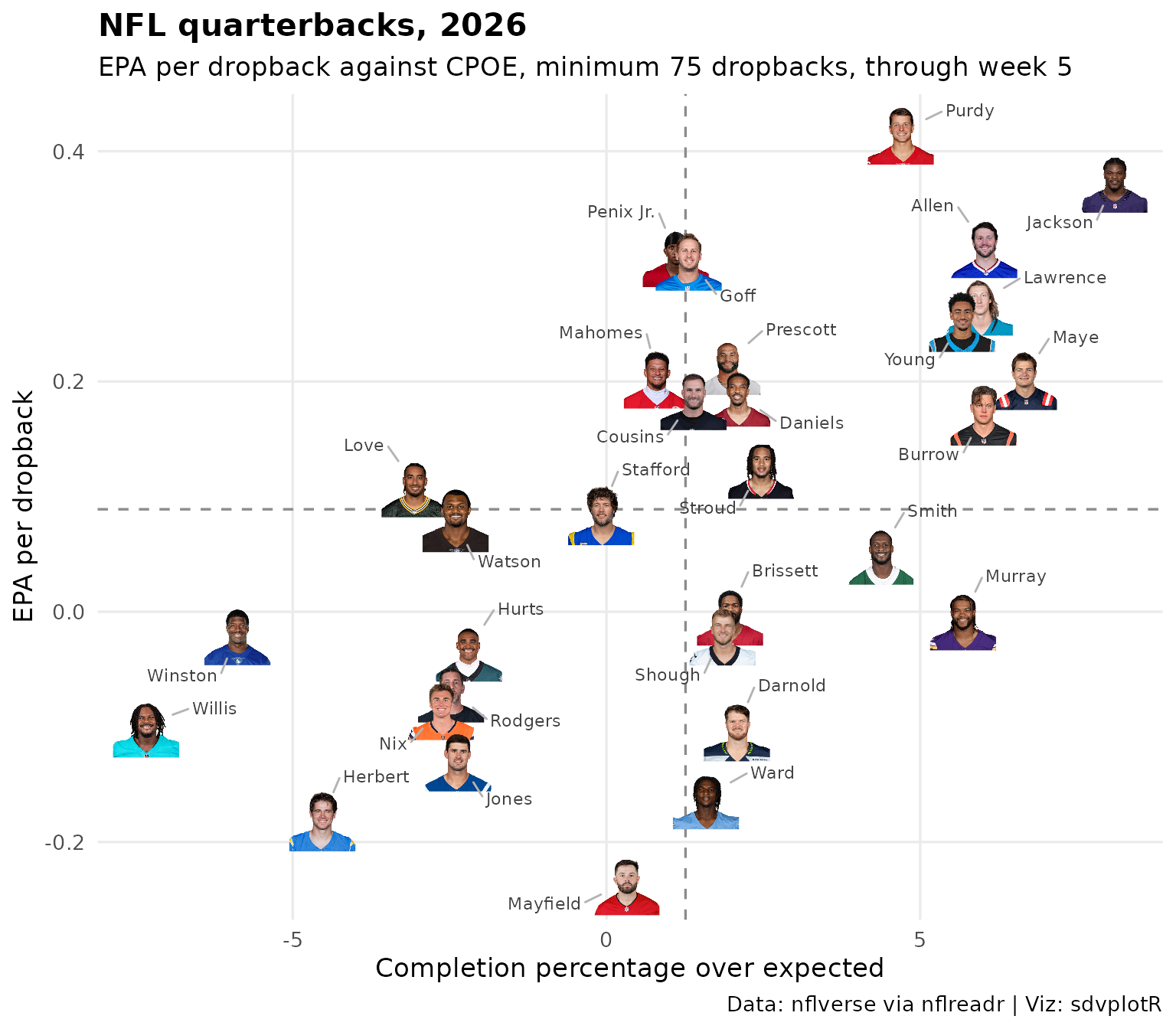

Every qualifying NFL quarterback's headshot placed by completion percentage over expected (horizontal) and EPA per dropback (vertical), with dashed lines at the averages of the group.

4. Interactive version

The offense-against-defense chart from section 2 as a plotly chart: hover a logo for the team’s record, EPA and rank, and drag a box to zoom into a crowded corner. A transparent marker trace carries the hover text, and add_sdv_logos() puts the logos on as layout images, in data units. plotly sizes its axes from the markers only, so the ranges get a margin for the logos, and a range given high-to-low reverses the defense axis.

pad <- function(v) range(v) + c(-1, 1) * 0.08 * diff(range(v))
plotly::plot_ly(
  power, x = ~off_epa, y = ~def_epa, type = "scatter", mode = "markers",
  marker = list(size = 24, opacity = 0), hoverinfo = "text",
  text = ~sprintf(
    "%s (%s), rank %d<br>Offense %+.3f, defense %+.3f<br>Net %+.3f per play",
    name, record, rank, off_epa, def_epa, net
  )
) |>
  plotly::layout(
    title = list(text = paste("NFL offense and defense,", season, through), x = 0.02),
    xaxis = list(title = "Offense: EPA per play", range = pad(power$off_epa)),
    yaxis = list(title = "Defense: EPA allowed per play (reversed)", range = rev(pad(power$def_epa)))
  ) |>
  add_sdv_logos(power$off_epa, power$def_epa, power$team, "nfl", size = 0.07)

More recipes like this one, in plotly, ggiraph, leaflet and reactable, are in Interactive charts.

Leaderboard Dashboards for layout patterns.
College football weekly, and the NBA, WNBA, MLB and NHL leaderboards.
Social graphics, automated posts tables like these on a schedule.

Our Authors

Citation

To cite the sdvplotR R package in publications, use:

BibTeX Citation

@misc{gilani_carl_lee_kay_weatherman_sdvplotR,
  author = {Gilani, Saiem and Carl, Sebastian and Lee, Jared and Kay, Camden and Weatherman, Andrew},
  title = {sdvplotR: The SportsDataverse's R Package for Multi-League Sports Plotting.},
  url = {https://sdvplotR.sportsdataverse.org},
  year = {2026}
}

sdvplot - the Python plotting package
sdvplot-js - the JavaScript / TypeScript plotting packages
cfbfastR - college football
hoopR - men’s basketball
wehoop - women’s basketball
baseballr - baseball
fastRhockey - hockey
oddsapiR - betting odds
sportyR - playing surfaces
sportsdataverse-py - the Python package
sportsdataverse-R - the R meta-package

Saiem Gilani