Percentile Bars and Cut Lines

Saiem Gilani

On this page

A table of numbers tells you the values. It does not tell you which ones stand out, where the line falls between one group and the next, or how far a row has moved. Three functions handle those jobs, and this article builds one table with each:

1. Percentile bars: the 2025 NFL season’s busiest quarterbacks, each one’s EPA per dropback and completion percentage over expected drawn against every qualified passer with gt_percentile_bar().
2. Cut lines: the NBA’s 2025-26 Western Conference standings, with gt_cutline() marking where the playoff seeds end and where the play-in ends.
3. Rank changes: the final 2025 college football AP Top 25 with each team’s move since the preseason poll, computed and colored by gt_delta().

The quarterbacks come from nflverse’s player stats via nflreadr, the standings from ESPN via hoopR and the polls from CollegeFootballData.com via cfbfastR (which needs a free API key). The three functions come from Andrew Weatherman’s gtUtils, and the first two sections follow his delay-table example.

library(sdvplotR)
library(gt)
library(gtExtras)
library(dplyr)

1. Percentile bars

We take every quarterback with at least 250 dropbacks (pass attempts plus sacks) in the 2025 regular season and compute two rates: EPA per dropback and completion percentage over expected (CPOE). Each gets a percentile among all the qualified passers, so the fifteen busiest can be read against the whole group, not just against each other.

qbs <- nflreadr::load_player_stats(2025, summary_level = "reg") |>
  filter(position == "QB") |>
  mutate(dropbacks = attempts + sacks_suffered, epa_db = passing_epa / dropbacks) |>
  filter(dropbacks >= 250) |>
  mutate(
    epa_ptile = cume_dist(epa_db),
    cpoe_ptile = cume_dist(passing_cpoe)
  ) |>
  arrange(desc(dropbacks), player_id) |>
  slice_head(n = 15) |>
  select(player_id, player_display_name, recent_team, dropbacks, epa_db, epa_ptile, passing_cpoe, cpoe_ptile)

cume_dist() gives each value’s percentile, on a 0-1 scale, which matters in a moment. Sorting on player_id after dropbacks breaks any tie the same way on every rebuild.

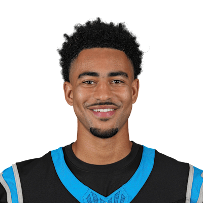
gt_percentile_bar() turns each percentile column into a filled track with a numbered marker at the tip. gt_sdv_headshots() turns the GSIS ids into NFL.com headshots and gt_sdv_logos() the team abbreviations into logos.

qbs |>
  gt(id = "qb-bars") |>
  gt_theme_almanac() |>
  gt_sdv_headshots(player_id, league = "nfl", id_system = "gsis", height = 34) |>
  gt_sdv_logos(recent_team, league = "nfl", height = 24) |>
  gt_percentile_bar(c(epa_ptile, cpoe_ptile), full_track = FALSE, width = 150) |>
  fmt_number(epa_db, decimals = 2, force_sign = TRUE) |>
  fmt_number(passing_cpoe, decimals = 1, force_sign = TRUE) |>
  tab_spanner(columns = c(epa_db, epa_ptile), "EPA per dropback") |>
  tab_spanner(columns = c(passing_cpoe, cpoe_ptile), "CPOE") |>
  cols_align(columns = -player_display_name, "center") |>
  gt_add_divider(dropbacks, color = "black", weight = px(1.5), include_labels = FALSE) |>
  cols_label(
    player_id = "", player_display_name = "Quarterback", recent_team = "",
    dropbacks = "Dropbacks", epa_db = "Value", epa_ptile = "Percentile",
    passing_cpoe = "Value", cpoe_ptile = "Percentile"
  ) |>
  tab_footnote(
    locations = cells_column_spanners(),
    footnote = "Percentile among every quarterback with at least 250 dropbacks in the 2025 regular season"
  ) |>
  tab_header(
    "The NFL's busiest passers, 2025",
    "The 15 quarterbacks with the most dropbacks, regular season"
  ) |>
  tab_source_note("Data: nflverse player stats via nflreadr")

The NFL's busiest passers, 2025
The 15 quarterbacks with the most dropbacks, regular season
	Quarterback		Dropbacks	EPA per dropback1		CPOE1
				Value	Percentile	Value	Percentile
	Bo Nix		634	+0.10	61	−1.2	27
	Dak Prescott		631	+0.18	88	+2.2	70
	Matthew Stafford		620	+0.24	97	+1.5	48
	Jared Goff		616	+0.17	85	+1.8	64
	Trevor Lawrence		601	+0.06	52	−1.9	24
	Cam Ward		595	−0.18	6	−2.9	12
	Caleb Williams		592	+0.07	58	−3.5	9
	Baker Mayfield		579	+0.00	27	−2.1	21
	Justin Herbert		566	+0.03	39	+1.6	52
	Drake Maye		539	+0.31	100	+10.8	100
	Patrick Mahomes		536	+0.13	67	+0.3	36
	Jacoby Brissett		528	−0.01	21	+1.6	58
	Aaron Rodgers		527	+0.05	48	+0.0	33
	Bryce Young		505	−0.04	18	+1.0	45
	Sam Darnold		504	+0.15	79	+5.2	91
1 Percentile among every quarterback with at least 250 dropbacks in the 2025 regular season
Data: nflverse player stats via nflreadr

The percentile columns are stored on a 0-1 scale, but the markers read as whole numbers out of 100. That is gt_percentile_bar()’s scale argument, which defaults to "auto": a column whose values all fall in [0, 1] is treated as a proportion and mapped onto the 0-100 axis, so a raw 0.71 prints as 71. A column already on a 0-100 scale is left alone, so the same code works either way. Set scale = "none" to turn that off.

The other arguments cover the look:

• domain: the value range the bar spans, c(0, 100) by default.
• palette: colors mapped across the domain, used for both the fill and the marker. The default runs blue at the low end through grey to red at the high end.
• full_track: whether the unfilled track runs the full width or stops at the marker. We set it to FALSE so each bar ends at its own value.
• width, marker_size, track_height, text_color, decimals: the column width, the marker, the thickness of the track, the color of the number inside the marker, and its decimal places.
• na_label: what to show for a missing percentile. It defaults to an em dash and draws a broken track, so an empty row cannot be misread as a percentile of zero.

The whole bar is CSS, not an image, so it stays sharp at any export size.

2. Cut lines

The second table asks where the lines fall in a standings table. In the NBA, seeds 1-6 in each conference go straight to the playoffs, seeds 7-10 play in for the last two places, and the rest go to the lottery. ESPN’s standings carry each team’s final seed, tiebreakers and the play-in applied, so the 7 and 8 seeds are the two play-in winners and the 8 seed can hold the better record.

nba_teams <- sdv_teams("nba")

west <- hoopR::espn_nba_standings(year = 2026) |>
  mutate(
    team_id = as.character(team_id),
    conference = nba_teams$conference[match(team_id, nba_teams$team_id)],
    abbr = nba_teams$abbr[match(team_id, nba_teams$team_id)]
  ) |>
  filter(conference == "Western Conference") |>
  arrange(playoffseed) |>
  transmute(
    seed = playoffseed, team = abbr, wins, losses,
    pct = winpercent, diff = as.numeric(differential), last_ten = lasttengames
  )

sdv_teams() gives each ESPN team id its conference and abbreviation; ESPN’s standings leave the conference out.

west |>
  gt(id = "west") |>
  gt_theme_almanac(accent = "#1D428A") |>
  gt_sdv_logos(team, league = "nba", height = 24) |>
  gt_cutline(after = 0, "Playoffs", color = "#1D428A") |>
  gt_cutline(after = 6, "Play-in", color = "#C8102E", gap = c(12, 0)) |>
  gt_cutline(after = 10, "Lottery", color = "#5A5A5A", gap = c(12, 0)) |>
  opt_row_striping(FALSE) |>
  fmt(pct, fns = function(x) sub("^0", "", sprintf("%.3f", x))) |>
  fmt_number(diff, decimals = 1, force_sign = TRUE) |>
  cols_label(
    seed = "Seed", team = "", wins = "W", losses = "L", pct = "Pct",
    diff = "Diff", last_ten = "Last 10"
  ) |>
  cols_align(columns = everything(), "center") |>
  tab_style(locations = cells_body(), style = cell_text(size = px(14))) |>
  tab_header(
    "Western Conference standings, 2025-26",
    "Regular-season records; final seeds, after the play-in. Diff is the average scoring margin."
  ) |>
  gt_538_caption(
    "Seeds 1-6 reach the playoffs; seeds 7-10 meet in the play-in for the last two places.",
    "Data: ESPN standings via hoopR"
  )

Western Conference standings, 2025-26
Regular-season records; final seeds, after the play-in. Diff is the average scoring margin.
Seed1	1	W1	L1	Pct1	Diff1	Last 101
1		64	18	.780	+11.1	7-3
2		62	20	.756	+8.3	8-2
3		54	28	.659	+5.2	10-0
4		53	29	.646	+1.7	7-3
5		52	30	.634	+5.2	9-1
6		49	33	.598	+3.4	5-5
7		42	40	.512	−0.3	7-3
8		45	37	.549	+1.5	5-5
9		42	40	.512	+1.2	6-4
10		37	45	.451	−0.6	3-7
11		26	56	.317	−4.5	1-9
12		26	56	.317	−5.5	3-7
13		25	57	.305	−6.0	1-9
14		22	60	.268	−10.0	3-7
15		22	60	.268	−8.4	1-9
1 Seeds 1-6 reach the playoffs; seeds 7-10 meet in the play-in for the last two places.
Data: ESPN standings via hoopR

There are three cut lines, one per group. gt_cutline(after = 6, ...) draws the rule between rows 6 and 7, where the playoff seeds give way to the play-in, and after = 10 does the same where the play-in ends. Each label sits on its line, rendered in uppercase.

The first call, gt_cutline(after = 0, ...), is the useful trick: after = 0 draws a line above the very first row, which labels the top section the same way the others are labelled.

A few arguments shape the lines:

• color, weight, style: the color, thickness, and line style ("dashed", "solid", or "dotted").
• label, label_position, label_size, label_color: the text on the line, whether it sits above or below, and how it looks.
• gap: extra space around the line, in pixels. A single number pads both sides; a length-2 vector c(above, below) sets them separately. Here gap = c(12, 0) opens room above each lower line without pushing the row below it down.

Note cell_text(size = px(14)) on the body: the gt_theme_* functions set their font sizes per cell, so tab_options(table.font.size = ...) will not move them. Restyle the body cells directly instead.

Cut lines are positional, not data-driven. gt::tab_row_group() splits a table on a value in the data and adds heading rows; a cut line leaves the table flowing and marks a fixed row number, which is what a standings table wants.

3. Rank changes

The last table puts a final ranking next to where each team started. The preseason AP poll is week 1 of the regular season in CollegeFootballData.com’s rankings, and the final poll is the only poll of the postseason. The polls need a CollegeFootballData.com key in CFBD_API_KEY; without one, or once its monthly calls are spent, this section’s code is shown but not run.

# a key with calls left this month (a margin for the articles built after this one): CFBD answers HTTP 429 with no rows once they are spent
has_key <- isTRUE(tryCatch(cfbfastR::cfbd_api_key_info()$remaining_calls > 10, error = function(e) FALSE))

ap_poll <- function(...) {
  cfbfastR::cfbd_rankings(year = 2025, ...) |>
    filter(poll == "AP Top 25") |>
    select(school, conference, rank)
}

preseason <- ap_poll(week = 1, season_type = "regular")
final <- ap_poll(season_type = "postseason")

moves <- final |>
  left_join(select(preseason, school, preseason = rank), by = "school") |>
  arrange(rank) |>
  select(rank, school, conference, preseason)

gt_delta(from, to) adds a column holding to - from, signed and colored by direction. For a ranking, a lower number is better, so passing the final rank as from and the preseason rank as to gives the places a team climbed: positive when it rose. A team that was unranked in the preseason has no starting rank, so its change is left blank and its preseason cell reads NR.

moves |>
  gt(id = "ap-moves") |>
  gt_theme_almanac(accent = "#9E1B32") |>
  gt_sdv_logos(school, league = "cfb", height = 22, include_name = TRUE) |>
  gt_delta(rank, preseason, column_label = "Places climbed", decimals = 0, arrows = TRUE) |>
  sub_missing(preseason, missing_text = "NR") |>
  cols_label(rank = "Final", school = "Team", conference = "Conference", preseason = "Preseason") |>
  cols_align(columns = -c(school, conference), "center") |>
  tab_style(locations = cells_body(), style = cell_text(size = px(14))) |>
  tab_header(
    "The final 2025 AP Top 25, and where each team started",
    "Final poll after the national championship, against the preseason poll"
  ) |>
  tab_source_note("Data: CollegeFootballData.com via cfbfastR")

The final 2025 AP Top 25, and where each team started
Final poll after the national championship, against the preseason poll
Final	Team	Conference	Preseason	Places climbed
1	Indiana	Big Ten	20	▲ 19
2	Miami	ACC	10	▲ 8
3	Ole Miss	SEC	21	▲ 18
4	Oregon	Big Ten	7	▲ 3
5	Ohio State	Big Ten	3	▼ 2
6	Georgia	SEC	5	▼ 1
7	Texas Tech	Big 12	23	▲ 16
8	Texas A&M	SEC	19	▲ 11
9	Alabama	SEC	8	▼ 1
10	Notre Dame	FBS Independents	6	▼ 4
11	BYU	Big 12	NR
12	Texas	SEC	1	▼ 11
13	Oklahoma	SEC	18	▲ 5
14	Utah	Big 12	NR
15	Vanderbilt	SEC	NR
16	Virginia	ACC	NR
17	Iowa	Big Ten	NR
18	Tulane	American Athletic	NR
19	James Madison	Sun Belt	NR
20	USC	Big Ten	NR
21	Michigan	Big Ten	14	▼ 7
22	Houston	Big 12	NR
23	Navy	American Athletic	NR
24	North Texas	American Athletic	NR
25	TCU	Big 12	NR
Data: CollegeFootballData.com via cfbfastR

arrows = TRUE leads each value with a triangle in place of a sign, so a fall reads as a down triangle in front of a positive number. With percent = TRUE the change is shown as a percent of from instead, which suits values such as points or yards better than ranks.

Our Authors

• Saiem Gilani
  
• Sebastian Carl
  
• Jared Lee
  
• Camden Kay
  
• Andrew Weatherman (gtUtils)
  

Citation

To cite the sdvplotR R package in publications, use:

BibTeX Citation

@misc{gilani_carl_lee_kay_weatherman_sdvplotR,
  author = {Gilani, Saiem and Carl, Sebastian and Lee, Jared and Kay, Camden and Weatherman, Andrew},
  title = {sdvplotR: The SportsDataverse's R Package for Multi-League Sports Plotting.},
  url = {https://sdvplotR.sportsdataverse.org},
  year = {2026}
}

Related SportsDataverse packages

• sdvplot - the Python plotting package
• sdvplot-js - the JavaScript / TypeScript plotting packages
• cfbfastR - college football
• hoopR - men’s basketball
• wehoop - women’s basketball
• baseballr - baseball
• fastRhockey - hockey
• oddsapiR - betting odds
• sportyR - playing surfaces
• sportsdataverse-py - the Python package
• sportsdataverse-R - the R meta-package