reactable and reactablefmtr cookbook
Saiem Gilani


Source: vignettes/cookbook-reactable.Rmd
cookbook-reactable.RmdOn this page
reactable makes
sortable, searchable tables for the web, and reactablefmtr adds
ready-made cell formats on top of it: data bars, color tiles, icon sets,
pill buttons, merged columns, embedded images and table themes.
sdvplotR’s reactable_sdv_*() helpers supply the team side:
logos, wordmarks, headshots and team colors, resolved from the same team
keys as the rest of the package. Recipes 1 to 6 combine the two
packages; recipes 7 to 10 use reactable alone for things the reactable integration article does
not show.
reactablefmtr is not an sdvplotR dependency. Install it from GitHub:
remotes::install_github("kcuilla/reactablefmtr")
library(sdvplotR)
library(reactable)
library(reactablefmtr)
library(dplyr, warn.conflicts = FALSE)
library(ggplot2)
Every table below is one row per team or player, aggregated from the season’s box scores or schedules, so a page embeds a few kilobytes of data rather than the play-by-play.
1. NBA: data bars in each team’s color
data_bars() draws a bar in each cell, and
fill_color_ref names a column that holds each row’s bar
color. sdv_team_colors() fills that column with each team’s
primary color, so the bars carry the same colors as the logos. The color
column is hidden with show = FALSE.
nba_box <- hoopR::load_nba_team_box(2026) |>
  filter(season_type == 2)

nba <- nba_box |>
  group_by(team = team_abbreviation, team_id) |>
  summarise(
    games = n(),
    wins = sum(team_score > opponent_team_score),
    ppg = mean(team_score),
    opp_ppg = mean(opponent_team_score),
    .groups = "drop"
  ) |>
  # drops the All-Star games; the NBA Cup final, which the standings do not
  # count, stays in the two finalists' lines
  filter(games >= 70) |>
  mutate(margin = ppg - opp_ppg, color = sdv_team_colors("nba", team)) |>
  arrange(desc(margin))
stopifnot(nrow(nba) == 30)
reactable(
  select(nba, team, wins, ppg, opp_ppg, margin, color),
  defaultPageSize = 10,
  columns = list(
    team = colDef(name = "", cell = reactable_sdv_logos(league = "nba", height = 26), html = TRUE, width = 60),
    wins = colDef(name = "W", width = 60),
    ppg = colDef(name = "PPG", format = colFormat(digits = 1), width = 70),
    opp_ppg = colDef(name = "Opp PPG", format = colFormat(digits = 1), width = 80),
    margin = colDef(
      name = "Point margin per game",
      cell = data_bars(nba, fill_color_ref = "color", number_fmt = scales::label_number(0.1, style_positive = "plus"))
    ),
    color = colDef(show = FALSE)
  )
)
A team with a negative margin gets a bar to the left of the zero line, so the table splits into winners and losers at a glance.
2. WNBA: a heatmap of team stats with
color_tiles()
color_tiles() fills each cell by its value in the
column, the same scale for every row. Pass it the column’s colors from
low to high; turnovers and points allowed get the reversed scale, so
green always means better. The team column uses
reactable_sdv_logos().
wnba <- wehoop::load_wnba_team_box(2025) |>
  filter(season_type == 2) |>
  group_by(team = team_abbreviation) |>
  summarise(
    games = n(),
    pts = mean(team_score),
    opp_pts = mean(opponent_team_score),
    fg_pct = sum(field_goals_made) / sum(field_goals_attempted),
    fg3_pct = sum(three_point_field_goals_made) / sum(three_point_field_goals_attempted),
    reb = mean(total_rebounds),
    ast = mean(assists),
    tov = mean(turnovers),
    .groups = "drop"
  ) |>
  filter(games >= 20) |> # drops the All-Star teams' single game
  arrange(desc(pts - opp_pts)) |>
  select(-games)

good <- c("#d7301f", "#fdf6e3", "#1a9850") # low to high, high is good
bad <- rev(good)
pct <- colFormat(percent = TRUE, digits = 1)
num <- scales::label_number(0.1)

reactable(
  wnba,
  pagination = FALSE,
  defaultColDef = colDef(width = 72),
  columns = list(
    team = colDef(name = "", cell = reactable_sdv_logos(league = "wnba", height = 26), html = TRUE, width = 60),
    pts = colDef(name = "PTS", cell = color_tiles(wnba, colors = good, number_fmt = num)),
    opp_pts = colDef(name = "OPP", cell = color_tiles(wnba, colors = bad, number_fmt = num)),
    fg_pct = colDef(name = "FG%", cell = color_tiles(wnba, colors = good, number_fmt = scales::label_percent(0.1))),
    fg3_pct = colDef(name = "3P%", cell = color_tiles(wnba, colors = good, number_fmt = scales::label_percent(0.1))),
    reb = colDef(name = "REB", cell = color_tiles(wnba, colors = good, number_fmt = num)),
    ast = colDef(name = "AST", cell = color_tiles(wnba, colors = good, number_fmt = num)),
    tov = colDef(name = "TOV", cell = color_tiles(wnba, colors = bad, number_fmt = num))
  )
)
3. NFL: player, team and headshot in one cell row with
merge_column()
merge_column() writes a second column’s value under (or
beside) the cell’s own, so the quarterback’s team abbreviation sits in
small grey type under his name and the table needs one column fewer. The
headshot comes from reactable_sdv_headshots(), which reads
nflverse’s GSIS ids, and the logo from
reactable_sdv_logos().
qbs <- nflreadr::load_player_stats(2025, summary_level = "reg") |>
  filter(position == "QB", attempts >= 250) |>
  transmute(
    player_id, player = player_display_name, team = recent_team, logo = recent_team,
    games, attempts,
    epa_per_play = passing_epa / (attempts + sacks_suffered),
    cpoe = passing_cpoe,
    td = passing_tds, int = passing_interceptions
  ) |>
  arrange(desc(epa_per_play))
stopifnot(!anyDuplicated(qbs$player_id))

reactable(
  qbs,
  defaultPageSize = 12,
  columns = list(
    player_id = colDef(
      name = "", width = 60, html = TRUE,
      cell = reactable_sdv_headshots(league = "nfl", id_system = "gsis", height = 40)
    ),
    player = colDef(name = "Quarterback", minWidth = 160, cell = merge_column(qbs, merged_name = "team", merged_position = "below")),
    team = colDef(show = FALSE),
    logo = colDef(name = "", cell = reactable_sdv_logos(league = "nfl", height = 28), html = TRUE, width = 56),
    games = colDef(name = "G", width = 50),
    attempts = colDef(name = "Att", width = 60),
    epa_per_play = colDef(name = "EPA/play", format = colFormat(digits = 3), width = 90),
    cpoe = colDef(name = "CPOE", format = colFormat(digits = 1), width = 70),
    td = colDef(name = "TD", width = 50),
    int = colDef(name = "INT", width = 50)
  )
)
4. MLB: run differential with icon_sets() and division
pill_buttons()
icon_sets() puts an icon before each number, picked by
the value’s third of the column: an up arrow for the best third, a dash
for the middle and a down arrow for the worst.
pill_buttons() turns a text column into a rounded tag;
color_ref points at a column of colors, here each team’s
primary color, so the tag reads as the team’s.
mlb_clubs <- baseballr::mlb_teams(season = 2025, sport_ids = 1) |>
  select(team_id, team = team_abbreviation, division = division_name, venue_id)

mlb_standings <- baseballr::mlb_standings(season = 2025, league_id = "103,104") |>
  transmute(
    team_id = team_records_team_id,
    w = team_records_wins,
    l = team_records_losses,
    rs = team_records_runs_scored,
    ra = team_records_runs_allowed,
    run_diff = team_records_run_differential
  )
stopifnot(identical(class(mlb_clubs$team_id), class(mlb_standings$team_id))) # same key type on both sides

mlb <- inner_join(mlb_clubs, mlb_standings, by = "team_id") |>
  mutate(
    division = sub("^American League", "AL", sub("^National League", "NL", division)),
    color = sdv_team_colors("mlb", team)
  ) |>
  arrange(desc(run_diff))
stopifnot(nrow(mlb) == 30)
reactable(
  select(mlb, team, division, w, l, rs, ra, run_diff, color),
  defaultPageSize = 10,
  columns = list(
    team = colDef(name = "", cell = reactable_sdv_logos(league = "mlb", height = 26), html = TRUE, width = 60),
    division = colDef(name = "Division", cell = pill_buttons(mlb, color_ref = "color", opacity = 0.85), minWidth = 110),
    w = colDef(name = "W", width = 55),
    l = colDef(name = "L", width = 55),
    rs = colDef(name = "RS", width = 60),
    ra = colDef(name = "RA", width = 60),
    run_diff = colDef(
      name = "Run diff",
      cell = icon_sets(mlb, icons = c("arrow-down", "minus", "arrow-up"), colors = c("#d7301f", "grey60", "#1a9850")),
      minWidth = 100
    ),
    color = colDef(show = FALSE)
  )
)
5. MLB: compare a team’s logo variants with
embed_img()
embed_img() draws a column that already holds image
URLs. sdv_logo_url() returns the URL of any variant
sdv_marks() lists, so one table can set a team’s variants
side by side, for picking the right one for a dark slide or a scoreboard
graphic. The dark variants sit on a dark cell background, where they are
meant to be read.
variants <- mlb |>
  slice_head(n = 8) |>
  transmute(
    team,
    default = sdv_logo_url(team, league = "mlb"),
    cap = sdv_logo_url(team, league = "mlb", variant = "cap_on_light"),
    dark = sdv_logo_url(team, league = "mlb", variant = "dark"),
    cap_dark = sdv_logo_url(team, league = "mlb", variant = "cap_on_dark")
  )

on_dark <- list(background = "#1d1d1f")
reactable(
  variants,
  pagination = FALSE,
  defaultColDef = colDef(align = "center", width = 110),
  columns = list(
    team = colDef(name = "Team", width = 70),
    default = colDef(name = "Default", cell = embed_img(height = 44)),
    cap = colDef(name = "Cap", cell = embed_img(height = 44)),
    dark = colDef(name = "Dark", cell = embed_img(height = 44), style = on_dark),
    cap_dark = colDef(name = "Cap on dark", cell = embed_img(height = 44), style = on_dark)
  )
)
embed_img() writes no alt text and has no
fallback when a URL is missing; the reactable_sdv_logos()
helper does both, so use embed_img() for this kind of
side-by-side review and the sdvplotR helper in tables readers see.
6. College football: a leaderboard with a reactablefmtr theme
reactablefmtr ships whole-table themes: espn(),
nytimes(), fivethirtyeight(),
pff() and more. One theme = argument sets the
fonts, borders, header and hover styles. This one ranks the 25 FBS teams
with the best scoring margin, from ESPN’s schedule data in cfbfastR’s
release files (no API key). ESPN team ids go straight to
reactable_sdv_logos(), and
reactable_sdv_team_color_bar() draws the margin bar in each
team’s color.
cfb_games <- cfbfastR::load_espn_cfb_schedules(2025) |>
  filter(season_type == 2, !is.na(home_score), !is.na(away_score))

cfb_side <- function(g, side, other) {
  transmute(g,
    team_id = as.character(.data[[paste0(side, "_id")]]),
    team = .data[[paste0(side, "_team")]],
    pts = .data[[paste0(side, "_score")]],
    opp = .data[[paste0(other, "_score")]]
  )
}
fbs <- sdv_teams("cfb")$team_id # sdvplotR's FBS and FCS programs, by ESPN id

cfb <- bind_rows(cfb_side(cfb_games, "home", "away"), cfb_side(cfb_games, "away", "home")) |>
  group_by(team_id, team) |>
  summarise(g = n(), w = sum(pts > opp), l = sum(pts < opp), margin = mean(pts - opp), .groups = "drop") |>
  filter(g >= 10, team_id %in% fbs) |>
  arrange(desc(margin)) |>
  slice_head(n = 25) |>
  mutate(rank = row_number(), logo = team_id, .before = 1)
reactable(
  select(cfb, rank, logo, team, w, l, margin),
  theme = espn(),
  defaultPageSize = 25,
  columns = list(
    rank = colDef(name = "#", width = 45),
    logo = colDef(name = "", cell = reactable_sdv_logos(league = "cfb", height = 26), html = TRUE, width = 50),
    team = colDef(name = "Team", minWidth = 140),
    w = colDef(name = "W", width = 50),
    l = colDef(name = "L", width = 50),
    margin = colDef(
      name = "Margin per game", minWidth = 150,
      format = colFormat(digits = 1),
      style = reactable_sdv_team_color_bar(cfb, "team_id", league = "cfb")
    )
  )
)
Swap espn() for nytimes() or
fivethirtyeight() and the same table takes that site’s
look.
7. NFL: wordmarks with reactable_sdv_wordmarks()
A wordmark is the team’s name as it is lettered on the uniform and
the stadium. reactable_sdv_wordmarks() draws it from the
same team key as reactable_sdv_logos(), with the same
height, variant and fallback rules. Wordmarks
are wide, so give the column room. Here it heads a division standings
table built from nflreadr’s schedules.
nfl_teams <- nflreadr::load_teams() |> select(team = team_abbr, division = team_division)
nfl <- nflreadr::load_schedules(2025) |>
  filter(game_type == "REG", !is.na(result)) |>
  nflreadr::clean_homeaway() |>
  group_by(team) |>
  summarise(
    w = sum(team_score > opponent_score),
    l = sum(team_score < opponent_score),
    t = sum(team_score == opponent_score),
    pf = sum(team_score), pa = sum(opponent_score),
    .groups = "drop"
  ) |>
  inner_join(nfl_teams, by = "team") |>
  mutate(logo = team, wordmark = team) |>
  arrange(division, desc(w + t / 2), desc(pf - pa))
stopifnot(nrow(nfl) == 32)

reactable(
  filter(nfl, division %in% c("AFC North", "NFC West")) |> select(division, logo, wordmark, w, l, t, pf, pa),
  pagination = FALSE,
  columns = list(
    division = colDef(name = "Division", width = 100),
    logo = colDef(name = "", cell = reactable_sdv_logos(league = "nfl", height = 30), html = TRUE, width = 56),
    wordmark = colDef(name = "", cell = reactable_sdv_wordmarks(league = "nfl", height = 24), html = TRUE, minWidth = 170),
    w = colDef(name = "W", width = 50), l = colDef(name = "L", width = 50), t = colDef(name = "T", width = 50),
    pf = colDef(name = "PF", width = 60), pa = colDef(name = "PA", width = 60)
  )
)
Logos in the column headers suit a head-to-head grid:
reactable_sdv_cols_label() turns every column named for a
team into a logo header. Each cell is the row team’s point margin
against the column team, summed over their two division games.
nfc_west <- c("LA", "SEA", "SF", "ARI")
h2h <- nflreadr::load_schedules(2025) |>
  filter(game_type == "REG", !is.na(result)) |>
  nflreadr::clean_homeaway() |>
  filter(team %in% nfc_west, opponent %in% nfc_west) |>
  group_by(team, opponent) |>
  summarise(margin = sum(team_score - opponent_score), .groups = "drop") |>
  tidyr::pivot_wider(names_from = opponent, values_from = margin) |>
  select(team, all_of(nfc_west)) |>
  slice(match(nfc_west, team))

reactable(
  h2h,
  columns = c(
    list(team = colDef(name = "", cell = reactable_sdv_logos(league = "nfl", height = 30), html = TRUE, width = 60)),
    reactable_sdv_cols_label(select(h2h, -team), league = "nfl", height = 30, align = "center", na = "")
  )
)
8. Men’s college basketball: teams grouped by conference
groupBy folds the rows into one row per value of a
column, and each column’s aggregate says how to summarise a
group: "mean", "max", "count" and
others. Click a conference to open its teams. The ratings are hoopR’s
adjusted efficiency margins for the 2025-26 season; each team’s
conference is the one ESPN’s standings list for that season, and the
join keeps the Division I teams (the ratings also hold the
lower-division teams they played once). hoopR stores the ratings’ team
id as text and the standings’ as a number, so both are made text before
the join.
mbb_ratings <- hoopR::load_mbb_ratings(2026) |>
  filter(season == 2026) |>
  transmute(team_id = as.character(team_id), adj_o, adj_d, adj_em)

mbb_conf <- hoopR::load_mbb_standings(2026) |>
  # ESPN also lists the College Basketball Crown, a postseason event, as a group
  filter(group_short_name != "CBC") |>
  distinct(team_id = as.character(team_id), team = team_short_display_name, conference = group_short_name)
stopifnot(identical(class(mbb_ratings$team_id), class(mbb_conf$team_id)), !anyDuplicated(mbb_conf$team_id))

mbb <- inner_join(mbb_conf, mbb_ratings, by = "team_id") |>
  mutate(logo = team_id) |>
  arrange(desc(adj_em))
reactable(
  select(mbb, conference, logo, team, adj_o, adj_d, adj_em),
  groupBy = "conference",
  defaultSorted = list(adj_em = "desc"),
  defaultPageSize = 12,
  columns = list(
    conference = colDef(name = "Conference", minWidth = 130),
    logo = colDef(name = "", cell = reactable_sdv_logos(league = "mbb", height = 24), html = TRUE, width = 50),
    team = colDef(name = "Teams", aggregate = "count", minWidth = 120),
    adj_o = colDef(name = "Adj. off.", aggregate = "mean", format = colFormat(digits = 1)),
    adj_d = colDef(name = "Adj. def.", aggregate = "mean", format = colFormat(digits = 1)),
    adj_em = colDef(name = "Adj. margin", aggregate = "mean", format = colFormat(digits = 1))
  )
)
Sorting by the adjusted margin sorts the conferences by their teams’ mean, so the strongest conference is on top before any group is opened.
9. Conference logos in cells
sdvplotR keeps the college conferences’ marks beside the teams’, and
the logo helpers resolve a conference by its short name, full name or
abbreviation ("Big East",
"Big East Conference").
sdv_teams("mbb", include_conferences = TRUE) lists them.
This table is one row per conference, with the conference’s logo and the
logo of its highest-rated team.
conferences <- mbb |>
  group_by(conference) |>
  summarise(
    teams = n(),
    mean_em = mean(adj_em),
    best = logo[which.max(adj_em)],
    best_em = max(adj_em),
    .groups = "drop"
  ) |>
  mutate(conf_logo = conference, .before = 1) |>
  arrange(desc(mean_em))

reactable(
  conferences,
  defaultPageSize = 12,
  columns = list(
    conf_logo = colDef(name = "", cell = reactable_sdv_logos(league = "mbb", height = 30), html = TRUE, width = 60),
    conference = colDef(name = "Conference", minWidth = 120),
    teams = colDef(name = "Teams", width = 70),
    mean_em = colDef(name = "Mean adj. margin", format = colFormat(digits = 1)),
    best = colDef(name = "Best team", cell = reactable_sdv_logos(league = "mbb", height = 28), html = TRUE, align = "center"),
    best_em = colDef(name = "Its margin", format = colFormat(digits = 1))
  )
)
10. NBA: expand a team to its players
details takes a function of the row index and returns
what to show when the row is opened, here a second reactable of that
team’s eight players with the most minutes, with ESPN headshots from
reactable_sdv_headshots(). Only the 240 player rows travel
with the page; the inner tables are built from them.
nba_players <- hoopR::load_nba_player_box(2026) |>
  filter(season_type == 2, !did_not_play, !is.na(minutes), team_abbreviation %in% nba$team) |>
  group_by(team = team_abbreviation, athlete_id, player = athlete_display_name) |>
  summarise(g = n(), min = mean(minutes), pts = mean(points), reb = mean(rebounds), ast = mean(assists), .groups = "drop") |>
  group_by(team) |>
  slice_max(g * min, n = 8, with_ties = FALSE) |>
  ungroup()

players_of <- function(abbr) {
  p <- filter(nba_players, team == abbr) |> select(athlete_id, player, g, min, pts, reb, ast)
  reactable(
    p,
    outlined = TRUE,
    defaultColDef = colDef(format = colFormat(digits = 1), width = 60),
    columns = list(
      athlete_id = colDef(name = "", cell = reactable_sdv_headshots(league = "nba", height = 36), html = TRUE, width = 56),
      player = colDef(name = "Player", minWidth = 150, width = NULL),
      g = colDef(name = "G", format = colFormat(digits = 0))
    )
  )
}

reactable(
  select(nba, team, wins, ppg, opp_ppg, margin),
  defaultPageSize = 10,
  details = function(index) players_of(nba$team[index]),
  columns = list(
    team = colDef(name = "", cell = reactable_sdv_logos(league = "nba", height = 28), html = TRUE, width = 60),
    wins = colDef(name = "W"),
    ppg = colDef(name = "PPG", format = colFormat(digits = 1)),
    opp_ppg = colDef(name = "Opp PPG", format = colFormat(digits = 1)),
    margin = colDef(name = "Margin", format = colFormat(digits = 1), style = reactable_sdv_team_color_bg(nba, "team", league = "nba"))
  )
)
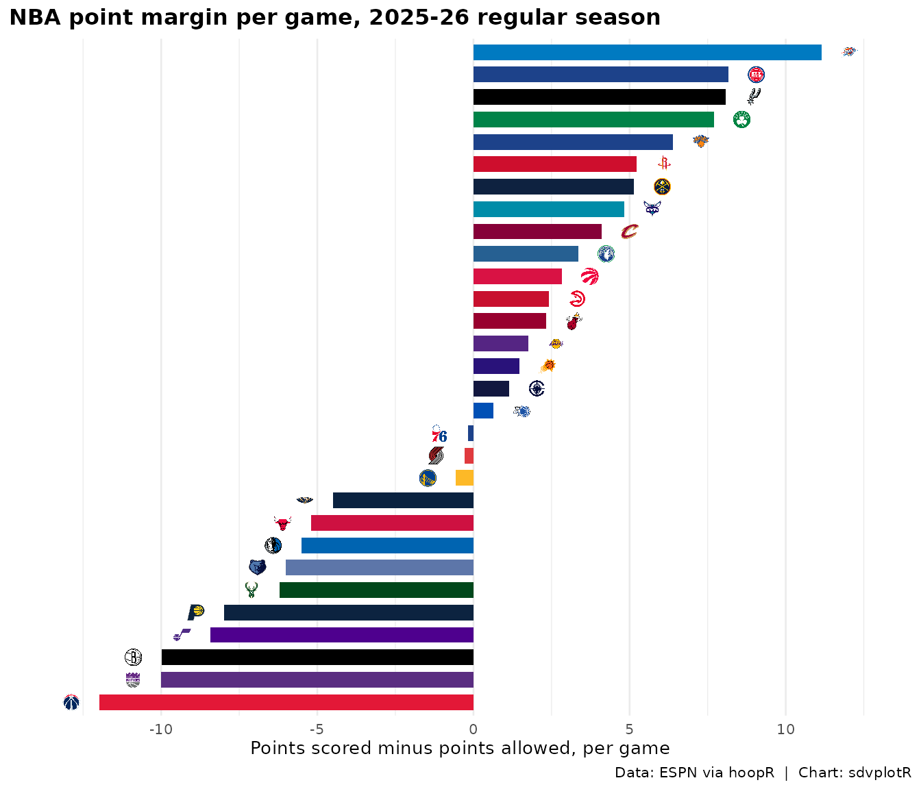
11. A static version for a post
A reactable is HTML, so it does not go into a slide or a social post
as it is. The first recipe’s numbers draw as a ggplot with the same team
colors: geom_col() takes each team’s color with
scale_fill_identity(), and geom_sdv_logos()
puts the logo at the end of each bar.
ggplot(nba, aes(margin, reorder(team, margin))) +
  geom_col(aes(fill = color), width = 0.7) +
  geom_sdv_logos(aes(team = team, x = margin + sign(margin) * 0.9), league = "nba", height = 0.028) +
  scale_fill_identity() +
  scale_x_continuous(expand = expansion(mult = 0.08)) +
  labs(
    title = "NBA point margin per game, 2025-26 regular season",
    x = "Points scored minus points allowed, per game", y = NULL,
    caption = "Data: ESPN via hoopR  |  Chart: sdvplotR"
  ) +
  theme_minimal(base_size = 10) +
  theme(
    plot.title.position = "plot",
    plot.title = element_text(face = "bold"),
    axis.text.y = element_blank(),
    panel.grid.major.y = element_blank()
  )
Related
-
reactable integration: the
reactable_sdv_*()helpers one at a time, with dark logos and headshots. - Interactive charts: ggiraph, plotly, leaflet and reactable with sdvplotR.
- Leaderboard dashboards: full leaderboards built on these tables.
- Reference: reactable_sdv_logos(), reactable_sdv_team_color_bar(), reactable_sdv_cols_label(), sdv_logo_url(), sdv_team_colors().


Related SportsDataverse packages
- sdvplot - the Python plotting package
- sdvplot-js - the JavaScript / TypeScript plotting packages
- cfbfastR - college football
- hoopR - men’s basketball
- wehoop - women’s basketball
- baseballr - baseball
- fastRhockey - hockey
- oddsapiR - betting odds
- sportyR - playing surfaces
- sportsdataverse-py - the Python package
- sportsdataverse-R - the R meta-package