
Interactive NHL Shot Map
Saiem Gilani


Source: vignettes/recipe-nhl-shot-map-interactive.Rmd
recipe-nhl-shot-map-interactive.RmdOn this page
The brief: the recap page for the Stanley Cup
clincher already carries the NHL Shot
Map image. The web version should let a reader point at any shot and
see who took it, when, what kind of shot it was and how it ended, with
the goals easy to find and each team’s logo at the end it attacks. The
data is the same SportsDataverse NHL release through fastRhockey;
sdv_surface() draws the rink, and ggiraph makes the ggplot
interactive without losing the rink or the logos.
library(sdvplotR)
library(ggplot2)
library(dplyr, warn.conflicts = FALSE)
library(ggiraph)

season <- 2026 # the 2025-26 season: NHL seasons are named by the year they end
cup_final <- 2025030416 # Stanley Cup Final, Game 6
1. Get the data
The same two loaders as the static recipe:
load_nhl_pbp() for the season’s play-by-play and
load_nhl_schedule() for the final score. This time each
shot keeps three more columns for the hover: the shot type
(secondary_type), the strength state and the distance.
pbp <- fastRhockey::load_nhl_pbp(season)
schedule <- fastRhockey::load_nhl_schedule(season)

game <- filter(schedule, game_id == cup_final)

shots <- pbp |>
  filter(game_id == cup_final, event_type %in% c("SHOT", "MISSED_SHOT", "GOAL")) |>
  transmute(
    event_type, period, period_time,
    team = event_team_abbr, shooter = event_player_1_name,
    shot_type = coalesce(secondary_type, "unknown"),
    strength_state, shot_distance,
    x_fixed, y_fixed, xg
  ) |>
  mutate(
    result = recode(event_type, SHOT = "Saved", MISSED_SHOT = "Missed", GOAL = "Goal"),
    id = row_number(),
    xg_label = if_else(is.na(xg), "xG not recorded", sprintf("xG %.2f", xg)),
    dot_size = coalesce(xg, min(xg, na.rm = TRUE)) # a shot without xG draws at the smallest size
  )
sprintf("%s %d at %s %d", game$away_team_abbr, game$away_score, game$home_team_abbr, game$home_score)
#> [1] "CAR 3 at VGK 0"
count(shots, team, result)
#> # A tibble: 5 × 3
#>   team  result     n
#>   <chr> <chr>  <int>
#> 1 CAR   Goal       3
#> 2 CAR   Missed    13
#> 3 CAR   Saved     20
#> 4 VGK   Missed    15
#> 5 VGK   Saved     22
sum(is.na(shots$xg))
#> [1] 1
The page embeds one row per shot, about a hundred rows, so it stays light. One saved shot has no expected-goals value in the release; it stays on the map at the smallest dot size, and its tooltip says so. Blocked shots are left out, as in the static recipe: the feed records where a blocked shot was blocked, not where it was taken.
The rink is the heavy part. sdv_surface() draws it with
‘sportyR’, whose curves (the corners, the circles, the creases) are
traced with over 120,000 points, many of them repeats a hundredth of a
foot apart. A static PNG doesn’t care, but girafe() writes
every point into the page, about 1.6 MB per chart. Dropping each point
that rounds to the same tenth of a foot as the one before it keeps about
one in six and leaves the drawing unchanged:
thin_rink <- function(rink) {
  rink$layers <- lapply(rink$layers, function(layer) {
    d <- layer$data
    if (is.data.frame(d) && all(c("x", "y") %in% names(d))) {
      key <- paste(round(d$x, 1), round(d$y, 1))
      layer$data <- d[c(TRUE, key[-1] != key[-length(key)]), ]
    }
    layer
  })
  rink
}

rink_points <- function(rink) sum(vapply(rink$layers, function(l) NROW(l$data), 1L))
c(before = rink_points(sdv_surface("nhl")), after = rink_points(thin_rink(sdv_surface("nhl"))))
#> before  after
#> 122424  20257
2. A tooltip on every shot
geom_point_interactive() is geom_point()
with three more aesthetics: tooltip (the HTML shown on
hover), data_id (which points light up together) and
onclick. The tooltip below names the shooter and his team,
the period and time, the shot type and strength, and how the shot ended.
The thinned sdv_surface("nhl") puts the shots on a rink
with the home team shooting right, and girafe() renders the
whole ggplot as an SVG.
shots <- mutate(
shots,
tip = sprintf(
"<b>%s</b> (%s)<br>Period %d, %s<br>%s shot, %s, %.0f ft<br>%s · %s",
shooter, team, period, period_time,
tools::toTitleCase(shot_type), strength_state, shot_distance, result, xg_label
)
)
p_tips <- thin_rink(sdv_surface("nhl")) +
geom_point_interactive(
aes(x_fixed, y_fixed, color = team, size = dot_size, tooltip = tip, data_id = id),
data = shots, alpha = 0.8
) +
scale_color_sdv(league = "nhl", guide = "none") +
scale_size_area(max_size = 4.5, guide = "none")
girafe(ggobj = p_tips, width_svg = 7, height_svg = 3.4)Every dot answers on hover, but a goal still looks like any other shot, and hovering one dot lights up only that dot.
3. Goals that stand out, shooters that light up
Three changes. Misses become open rings, saved shots stay filled
dots, and goals become large black-ringed dots drawn last so they sit on
top. data_id is now the shooter, so hovering a shot lights
up every shot that player took; the opts_hover_inv() option
fades everything else. A click keeps a shooter selected
(opts_selection()), for comparing where two players shot
from.
draw_shots <- function(...) {
  thin_rink(sdv_surface("nhl", ...)) +
    geom_point_interactive(
      aes(x_fixed, y_fixed, color = team, size = dot_size, tooltip = tip, data_id = shooter),
      data = filter(shots, result == "Saved"), alpha = 0.8
    ) +
    geom_point_interactive(
      aes(x_fixed, y_fixed, color = team, size = dot_size, tooltip = tip, data_id = shooter),
      data = filter(shots, result == "Missed"), shape = 1, stroke = 0.9
    ) +
    geom_point_interactive(
      aes(x_fixed, y_fixed, fill = team, tooltip = tip, data_id = shooter),
      data = filter(shots, result == "Goal"), shape = 21, size = 6.5, color = "black", stroke = 1.2
    ) +
    scale_color_sdv(league = "nhl", guide = "none") +
    scale_fill_sdv(league = "nhl", guide = "none") +
    scale_size_area(max_size = 4.5, guide = "none")
}

shot_opts <- list(
  opts_tooltip(css = "background:white;color:black;padding:6px;border-radius:6px;font-size:12px;"),
  opts_hover(css = "stroke:black;stroke-width:1.5px;"),
  opts_hover_inv(css = "opacity:0.15;"),
  opts_selection(type = "single", css = "stroke:black;stroke-width:2px;")
)

girafe(ggobj = draw_shots(), width_svg = 7, height_svg = 3.4, options = shot_opts)
4. Logos, score and headline
Each team gets its logo, score and shots on goal past the boards on
the side it attacks, as in the static recipe.
geom_sdv_logos_interactive() is
geom_sdv_logos() with a hover target over each logo, so the
logo gets its own tooltip: the full team name and the shot totals. Its
data_id is the team, which doesn’t match any shooter, so
hovering a logo highlights only that logo.
club_names <- sdv_teams("nhl") |> select(team_abbr = abbr, team_name = name)
scoreboard <- tibble(
  team = c(game$away_team_abbr, game$home_team_abbr),
  x = c(-122, 122), # outside the boards, on the side each team attacks
  score = c(game$away_score, game$home_score)
) |>
  left_join(
    summarise(shots, sog = sum(result != "Missed"), attempts = n(), xg = sum(xg, na.rm = TRUE), .by = team),
    by = "team"
  ) |>
  left_join(club_names, by = c("team" = "team_abbr")) |>
  mutate(tip = sprintf(
    "<b>%s</b><br>%d goals, %d shots on goal<br>%d unblocked attempts, %.1f xG",
    team_name, score, sog, attempts, xg
  ))
winner <- slice_max(scoreboard, score, n = 1)
loser <- slice_min(scoreboard, score, n = 1)

shot_map <- function() {
  draw_shots(xlims = c(-142, 142)) +
    geom_sdv_logos_interactive(
      aes(x = x, y = 14, team = team, tooltip = tip, data_id = team),
      data = scoreboard, league = "nhl", height = 0.2, hover_size = 14
    ) +
    geom_text(aes(x = x, y = -8, label = score), data = scoreboard, size = 11, fontface = "bold") +
    geom_text(
      aes(x = x, y = -21, label = paste(sog, "shots\non goal")),
      data = scoreboard, size = 2.7, color = "grey40", lineheight = 0.9
    ) +
    labs(
      title = sprintf(
        "The %s won the Stanley Cup, %d-%d in Game 6",
        winner$team_name, winner$score, loser$score
      ),
      subtitle = sprintf(
        "Every unblocked shot. %s shoots left, %s right. Dots: saved; rings: missed; large black-ringed dots: goals; size: expected goals.",
        game$away_team_abbr, game$home_team_abbr
      ),
      caption = "Data: NHL via fastRhockey  |  Chart: sdvplotR"
    ) +
    theme(
      plot.title = element_text(face = "bold", size = 14, margin = margin(b = 3)),
      plot.subtitle = ggtext::element_textbox_simple(color = "grey40", size = 8.5, margin = margin(b = 4)),
      plot.caption = element_text(color = "grey45", size = 7),
      plot.margin = margin(10, 12, 6, 12),
      plot.background = element_rect(fill = "white", color = NA)
    )
}

shot_widget <- girafe(ggobj = shot_map(), width_svg = 8, height_svg = 4.5, options = shot_opts)
shot_widget
The two logos are embedded in the SVG, so the chart needs no network once the page has loaded.
5. Share it
htmlwidgets::saveWidget() writes the widget to one HTML
file. selfcontained = TRUE inlines ggiraph’s JavaScript, so
the file opens anywhere with no folder beside it (it needs pandoc, which
ships with RStudio).
out_dir <- tempfile("sdvplotR-recipe-") # where the file goes; use your own folder
dir.create(out_dir)
html <- file.path(out_dir, "nhl_shot_map.html")
htmlwidgets::saveWidget(shot_widget, html, selfcontained = TRUE)
round(file.size(html) / 1024) # kilobytes
#> [1] 8869
6. A static version
The same plot without girafe() is an ordinary ggplot, so
a social post or a PDF gets the matching image: outside
girafe() the _interactive layers draw as plain
points and logos, and the hover targets stay invisible.
ggsave() it as in the NHL Shot Map recipe.
shot_map()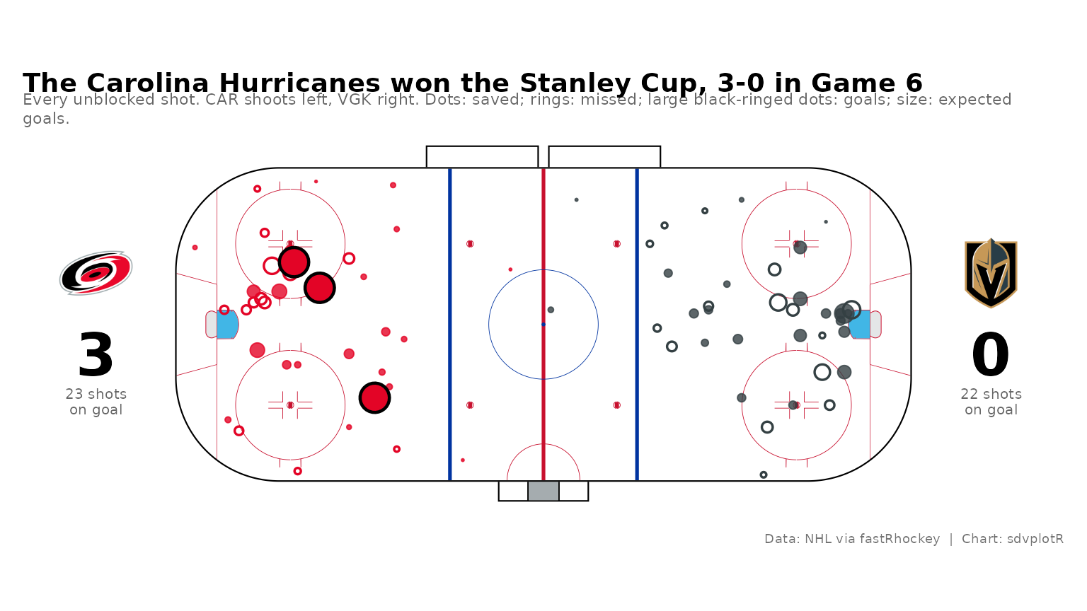
Related
- NHL Shot Map: the static recipe this page extends, with the 1200 x 675 and 1600 x 900 exports.
- Interactive charts: ggiraph, plotly, leaflet and reactable recipes.
- Reference:
sdv_surface(),geom_sdv_logos_interactive(),geom_sdv_logos(),scale_color_sdv().






Related SportsDataverse packages
- sdvplot - the Python plotting package
- sdvplot-js - the JavaScript / TypeScript plotting packages
- cfbfastR - college football
- hoopR - men’s basketball
- wehoop - women’s basketball
- baseballr - baseball
- fastRhockey - hockey
- oddsapiR - betting odds
- sportyR - playing surfaces
- sportsdataverse-py - the Python package
- sportsdataverse-R - the R meta-package