


On this page
A shot chart with one dot per attempt shows where a player shoots, but not whether he makes them more often than anyone else from there. This recipe cuts the half court into 3 ft squares and colors each square by the player’s field goal percentage minus the league’s from the same square. Busier squares are drawn more solid, and squares where the player took fewer than 5 attempts are left out, so no tile rests on one or two shots.
The court is drawn with ggplot2::annotate(), so the
recipe needs no court package. The colors are the team’s own, from
sdv_team_colors(), and the logo in the title comes from
ggtitle_image().
The data
hoopR’s load_nba_shots() reads the SportsDataverse
release of ESPN shot locations, one row per shot, free throws included.
Season 2026 is 2025-26.
shots <- as.data.frame(hoopR::load_nba_shots(2026))
dim(shots)
#> [1] 298411     20
names(shots)
#>  [1] "game_id"             "season"              "period_number"
#>  [4] "clock_display_value" "team_id"             "athlete_id_1"
#>  [7] "athlete_id_2"        "type_id"             "type_text"
#> [10] "scoring_play"        "score_value"         "coordinate_x"
#> [13] "coordinate_y"        "coordinate_x_raw"    "coordinate_y_raw"
#> [16] "athlete_name_1"      "athlete_name_2"      "team_name"
#> [19] "team_mascot"         "team_abbrev"
The file also holds the play-in and the playoffs.
load_nba_schedule() marks each game’s
season_type (2 is the regular season), so keep
those games, drop free throws, and drop heaves from past half court.
schedule <- as.data.frame(hoopR::load_nba_schedule(2026))
stopifnot(identical(class(shots$game_id), class(schedule$game_id)))
regular <- schedule$game_id[schedule$season_type == 2]

fga <- shots |>
  filter(
    game_id %in% regular,
    !grepl("Free Throw", type_text),
    coordinate_y_raw <= 41
  ) |>
  mutate(x = coordinate_x_raw - 25, y = coordinate_y_raw, made = scoring_play)
nrow(fga)
#> [1] 219514
coordinate_x_raw runs 0 to 50 ft across the court, so
the rim is at 25 and x is feet left or right of it.
coordinate_y_raw is feet from the rim toward half court,
with the baseline about 5 ft behind it. Two checks of that frame: dunks
should land about a foot from the rim, and no made three should be
closer than the 22 ft corner three (score_value is the
points a shot scored, so a made three has
score_value == 3).
dunks <- fga |> filter(grepl("Dunk", type_text))
threes <- fga |> filter(made, score_value == 3)
c(
  dunk_median_ft = median(sqrt(dunks$x^2 + dunks$y^2)),
  three_min_ft = min(sqrt(threes$x^2 + threes$y^2))
)
#> dunk_median_ft   three_min_ft
#>       1.414214      22.000000
stopifnot(
  median(sqrt(dunks$x^2 + dunks$y^2)) < 2,
  min(sqrt(threes$x^2 + threes$y^2)) >= 22
)
The grid
Round each shot to the centre of a 3 ft square, with one square centred on the rim. The league’s field goal percentage per square uses every regular-season attempt, the player’s included.
bin <- 3
fga <- fga |> mutate(bx = round(x / bin) * bin, by = round(y / bin) * bin)

league <- fga |>
  summarise(league_fg = mean(made), .by = c(bx, by))

shooter <- "Shai Gilgeous-Alexander"
grid <- fga |>
  filter(athlete_name_1 == shooter) |>
  summarise(attempts = n(), fg = mean(made), .by = c(bx, by)) |>
  left_join(league, by = c("bx", "by")) |>
  mutate(diff = fg - league_fg)

shown <- grid |> filter(attempts >= 5)
stopifnot(all(shown$attempts >= 5))
c(
  attempts = sum(grid$attempts),
  squares = nrow(grid),
  squares_shown = nrow(shown),
  attempts_shown = sum(shown$attempts)
)
#>       attempts        squares  squares_shown attempts_shown
#>           1323            141             79           1201
The court
NBA dimensions in feet, with the rim at (0, 0): the
three-point arc is 23.75 ft from the rim and 22 ft in the corners, the
lane is 16 ft wide, the free-throw line is 15 ft from the backboard, and
the restricted area is a 4 ft arc. The function returns a list of
layers, so it adds to a plot like any other layer.
court <- function(colour = "grey40", linewidth = 0.4) {
  arc <- function(r, from, to, y0 = 0) {
    a <- seq(from, to, length.out = 120)
    data.frame(x = r * cos(a), y = y0 + r * sin(a))
  }
  corner <- sqrt(23.75^2 - 22^2)
  three <- arc(23.75, atan2(corner, 22), pi - atan2(corner, 22))
  free_throw <- arc(6, 0, pi, y0 = 13.75)
  restricted <- arc(4, 0, pi)
  rim <- arc(0.75, 0, 2 * pi)
  line <- function(geom, ...) {
    annotate(geom, ..., colour = colour, linewidth = linewidth)
  }
  list(
    line("rect", xmin = -25, xmax = 25, ymin = -5.25, ymax = 41.75, fill = NA),
    line("rect", xmin = -8, xmax = 8, ymin = -5.25, ymax = 13.75, fill = NA),
    line("path", x = free_throw$x, y = free_throw$y),
    line("path", x = restricted$x, y = restricted$y),
    line("path", x = three$x, y = three$y),
    line("segment", x = c(-22, 22), xend = c(-22, 22), y = -5.25, yend = corner),
    line("segment", x = -3, xend = 3, y = -1.25, yend = -1.25),
    line("path", x = rim$x, y = rim$y)
  )
}
The plot
Tiles go under the court lines. The view stops 37 ft from the
baseline (31.75 ft past the rim), and the first line of the chunk checks
that every shown square fits inside it. The fill runs from the team’s
secondary color (below the league) through grey (level with it) to its
primary color (above it), capped at 20 points either way so one hot
corner does not wash out the rest. Alpha follows attempts. If a team’s
secondary color is close to grey or white, the “below” end would blur
into the midpoint: pass a darker color as below for that
team.
stopifnot(max(shown$by) + bin / 2 <= 31.75)
shooter_team <- unique(fga$team_abbrev[fga$athlete_name_1 %in% shooter])
shooter_team
#> [1] "OKC"
# a player traded mid-season has two teams: pick one before taking its colors
stopifnot(length(shooter_team) == 1)
above <- sdv_team_colors("nba", shooter_team, which = "primary")
below <- sdv_team_colors("nba", shooter_team, which = "secondary")

ggplot(shown) +
  geom_tile(
    aes(bx, by, fill = diff, alpha = attempts),
    width = bin, height = bin
  ) +
  court() +
  scale_fill_gradient2(
    low = below, mid = "grey85", high = above, midpoint = 0,
    limits = c(-0.2, 0.2), oob = scales::squish,
    labels = function(v) sprintf("%+.0f", 100 * v),
    name = "FG% vs league\n(points)"
  ) +
  scale_alpha_continuous(range = c(0.35, 1), name = "Attempts") +
  coord_fixed(xlim = c(-25, 25), ylim = c(-5.25, 31.75), expand = FALSE) +
  ggtitle_image(
    title_image = shooter_team,
    title = shooter,
    subtitle = "2025-26 regular season, 3 ft squares with 5+ attempts",
    image_height = 22,
    league = "nba"
  ) +
  labs(caption = "Data: hoopR::load_nba_shots()") +
  theme_void() +
  theme_title_image(size = 16) +
  theme(legend.position = "bottom", plot.margin = margin(8, 8, 8, 8))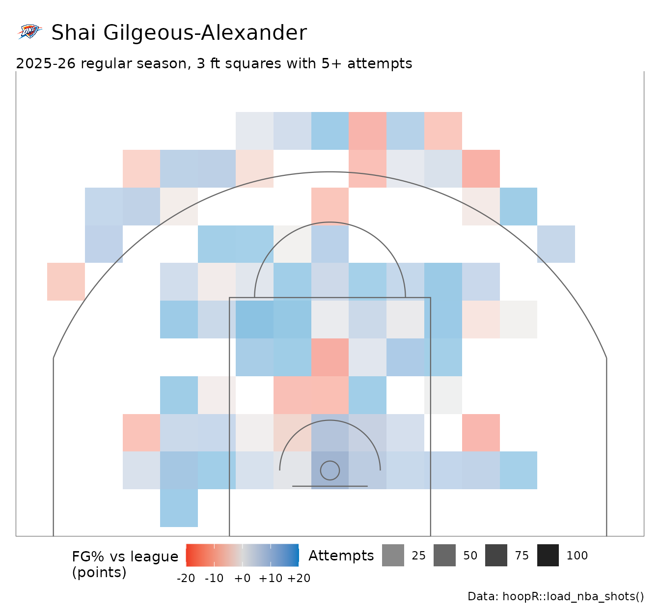






Related SportsDataverse packages
- sdvplot - the Python plotting package
- sdvplot-js - the JavaScript / TypeScript plotting packages
- cfbfastR - college football
- hoopR - men’s basketball
- wehoop - women’s basketball
- baseballr - baseball
- fastRhockey - hockey
- oddsapiR - betting odds
- sportyR - playing surfaces
- sportsdataverse-py - the Python package
- sportsdataverse-R - the R meta-package