
CFB Stadium Map
Saiem Gilani


Source: vignettes/recipe-cfb-stadium-map.Rmd
recipe-cfb-stadium-map.RmdOn this page
The brief: the preseason guide wants a map of
college football: every FBS program as its logo, sitting on its home
stadium, so a reader can find the schools near them, click one for its
stadium and capacity, and show one conference at a time. This recipe is
new, not the interactive version of a static one. The stadiums come from
CollegeFootballData.com through cfbfastR, leaflet draws the map, and
sdvplotR’s addSdvLogoMarkers() turns each marker into a
team logo.
CollegeFootballData.com needs a free API key in
CFBD_API_KEY (get one at https://collegefootballdata.com/key; see
?cfbfastR::register_cfbd). Without one, the code below is
shown but not run.
has_key <- nzchar(Sys.getenv("CFBD_API_KEY"))
if (!has_key) cat("CFBD_API_KEY is not set, so the chunks below are shown but not run.\n")
knitr::opts_chunk$set(eval = has_key)
library(sdvplotR)
library(dplyr, warn.conflicts = FALSE)
library(leaflet)
library(ggplot2)

season <- 2025
1. Get the data
cfbd_team_info() returns one row per school, and with
only_fbs = TRUE and a year it is that season’s
FBS teams with their conference and home venue: stadium name, city,
state, latitude, longitude and capacity. No join is needed. CFBD’s
team_id is ESPN’s team id, the id sdvplotR keys college
teams by, so it goes to the logo functions as it is. That skips name
matching, where "Charlotte" alone could be the 49ers or the
Saints.
stadiums <- cfbfastR::cfbd_team_info(only_fbs = TRUE, year = season) |>
  as.data.frame() |>
  transmute(
    team = as.character(team_id), school, conference,
    venue = venue_name, city, state, capacity,
    lon = longitude, lat = latitude
  ) |>
  arrange(conference, school)
nrow(stadiums)
#> [1] 136
count(stadiums, conference)
#>           conference  n
#> 1                ACC 17
#> 2  American Athletic 14
#> 3             Big 12 16
#> 4            Big Ten 18
#> 5     Conference USA 12
#> 6   FBS Independents  2
#> 7       Mid-American 13
#> 8      Mountain West 12
#> 9             Pac-12  2
#> 10               SEC 16
#> 11          Sun Belt 14
A popup is HTML, so the text that goes into it is escaped first
(Texas A&M has an ampersand):
esc <- htmltools::htmlEscape
stadiums <- stadiums |>
  mutate(popup = sprintf(
    "<b>%s</b><br>%s<br>%s<br>Capacity %s<br>%s, %s",
    esc(school), esc(conference), esc(venue), format(capacity, big.mark = ","), esc(city), state
  ))
2. The map
Start with the logos. addSdvLogoMarkers() reads the
coordinates and team ids from the map’s data with formulas, and
label is the text shown on hover. A light basemap keeps the
logos readable, and fitBounds() frames the continental
United States (Hawai’i is off the frame; zoom out to find it).
lower48 <- c(-125, 24, -66.5, 49.5) # west, south, east, north

leaflet(stadiums) |>
  addProviderTiles(providers$CartoDB.Positron) |>
  addSdvLogoMarkers(~lon, ~lat, ~team, league = "cfb", size = 26, label = ~school) |>
  fitBounds(lower48[1], lower48[2], lower48[3], lower48[4])
Hover names the school. Add the popup, and a click opens the stadium details:
leaflet(stadiums) |>
  addProviderTiles(providers$CartoDB.Positron) |>
  addSdvLogoMarkers(~lon, ~lat, ~team, league = "cfb", size = 26, label = ~school, popup = ~popup) |>
  fitBounds(lower48[1], lower48[2], lower48[3], lower48[4])
The Southeast is crowded at this zoom. Put each conference’s markers
in its own leaflet group, and addLayersControl() lists the
groups with a checkbox each, so the reader can show one conference, or
compare two:
stadium_map <- leaflet() |>
  addProviderTiles(providers$CartoDB.Positron)
for (conf in unique(stadiums$conference)) {
  stadium_map <- stadium_map |>
    addSdvLogoMarkers(
      ~lon, ~lat, ~team,
      league = "cfb", size = 26, label = ~school, popup = ~popup, group = conf,
      data = filter(stadiums, conference == conf)
    )
}
stadium_map <- stadium_map |>
  addLayersControl(
    overlayGroups = unique(stadiums$conference),
    options = layersControlOptions(collapsed = FALSE)
  ) |>
  fitBounds(lower48[1], lower48[2], lower48[3], lower48[4])
stadium_map
The map has no data of its own here, so each call passes its
conference’s rows with data =, and the formulas read
those.
3. Share it
htmlwidgets::saveWidget() writes the map to one HTML
file; selfcontained = TRUE inlines leaflet’s JavaScript, so
the file opens anywhere. The logos and map tiles stay links, so the file
needs the network when it is opened.
html <- tempfile("cfb-stadiums-", fileext = ".html")
htmlwidgets::saveWidget(stadium_map, html, selfcontained = TRUE, title = "FBS stadiums")
round(file.size(html) / 1024) # kilobytes
#> [1] 525
4. The static version
For a print page or a post, draw the same logos with ggplot2 at their
longitude and latitude over the state outlines from
map_data("state") (it needs the maps package).
coord_quickmap() keeps the map’s proportions. Hawai’i is
left out to keep the frame on the lower 48.
states <- map_data("state")
mainland <- filter(stadiums, state != "HI")

ggplot() +
  geom_polygon(
    data = states, aes(x = long, y = lat, group = group),
    fill = "grey97", colour = "grey75", linewidth = 0.2
  ) +
  geom_sdv_logos(data = mainland, aes(x = lon, y = lat, team = team), league = "cfb", height = 0.04) +
  coord_quickmap() +
  labs(
    title = paste("Every FBS program at its home stadium,", season),
    caption = "Data: CollegeFootballData.com via cfbfastR | Viz: sdvplotR"
  ) +
  theme_void() +
  theme(plot.title = element_text(face = "bold"))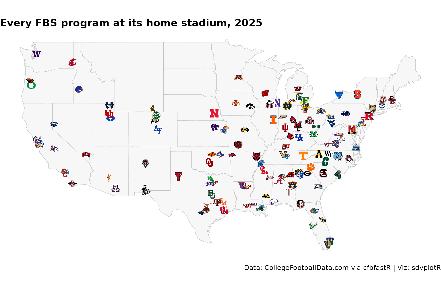
Related
- College Football: cfbfastR and sdvplotR across ten charts and tables.
- CFB Conference Table: a static recipe from the same data source.
- Interactive charts: ggiraph, plotly, leaflet and reactable with sdvplotR.
- Reference: addSdvLogoMarkers(), geom_sdv_logos().






Related SportsDataverse packages
- sdvplot - the Python plotting package
- sdvplot-js - the JavaScript / TypeScript plotting packages
- cfbfastR - college football
- hoopR - men’s basketball
- wehoop - women’s basketball
- baseballr - baseball
- fastRhockey - hockey
- oddsapiR - betting odds
- sportyR - playing surfaces
- sportsdataverse-py - the Python package
- sportsdataverse-R - the R meta-package